January 2016 – HCSE Blog

31/01/2016

The Magic Black Box

It was the appointed time for Bob and Leslie’s regular coaching session as part of the improvement science practitioner programme.

<Leslie> Hi Bob, I am feeling rather despondent today so please excuse me in advance if you hear a lot of “Yes, but …” language.

<Bob> I am sorry to hear that Leslie. Do you want to talk about it?

<Leslie> Yes, please. The trigger for my gloom was being sent on a mandatory training workshop.

<Bob> OK. Training to do what?

<Leslie> Outpatient demand and capacity planning!

<Bob> But you know how to do that already, so what is the reason you were “sent”?

<Leslie> Well, I am no longer sure I know how to it. That is why I am feeling so blue. I went more out of curiosity and I came away utterly confused and with my confidence shattered.

<Bob> Oh dear! We had better start at the beginning. What was the purpose of the workshop?

<Leslie> To train everyone in how to use an Outpatient Demand and Capacity planning model, an Excel one that we were told to download along with the User Guide. I think it is part of a national push to improve waiting times for outpatients.

<Bob> OK. On the surface that sounds reasonable. You have designed and built your own Excel flow-models already; so where did the trouble start?

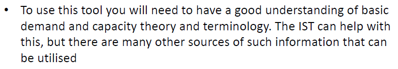
<Leslie> I will attempt to explain. This was a paragraph in the instructions. I felt OK with this because my Improvement Science training has given me a very good understanding of basic demand and capacity theory.

<Bob> OK. I am guessing that other delegates may have felt less comfortable with this. Was that the case?

<Leslie> The training workshops are targeted at Operational Managers and the ones I spoke to actually felt that they had a good grasp of the basics.

<Bob> OK. That is encouraging, but a warning bell is ringing for me. So where did the trouble start?

<Leslie> Well, before going to the workshop I decided to read the User Guide so that I had some idea of how this magic tool worked. This is where I started to wobble – this paragraph specifically …

<Bob> H’mm. What did you make of that?

<Leslie> It was complete gibberish to me and I felt like an idiot for not understanding it. I went to the workshop in a bit of a panic and hoped that all would become clear. It didn’t.

<Bob> Did the User Guide explain what ‘percentile’ means in this context, ideally with some visual charts to assist?

<Leslie> No and the use of ‘th’ and ‘%’ was really confusing too. After that I sort of went into a mental fog and none of the workshop made much sense. It was all about practising using the tool without any understanding of how it worked. Like a black magic box.

<Bob> OK. I can see why you were confused, and do not worry, you are not an idiot. It looks like the author of the User Guide has unwittingly used some very confusing and ambiguous terminology here. So can you talk me through what you have to do to use this magic box?

<Leslie> First we have to enter some of our historical data; the number of new referrals per week for a year; and the referral and appointment dates for all patients for the most recent three months.

<Bob> OK. That sounds very reasonable. A run chart of historical demand and the raw event data for a Vitals Chart® is where I would start the measurement phase too – so long as the data creates a valid 3 month reporting window.

<Leslie> Yes, I though so too … but that is not how the black box model seems to work. The weekly demand is used to draw an SPC chart, but the event data seems to disappear into the innards of the black box, and recommendations pop out of it.

<Bob> Ah ha! And let me guess the relationship between the term ‘percentile’ and the SPC chart of weekly new demand was not explained?

<Leslie> Spot on. What does percentile mean?

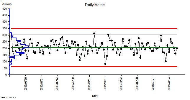
<Bob> It is statistics jargon. Remember that we have talked about the distribution of the data around the average on a BaseLine chart; and how we use the histogram feature of BaseLine to show it visually. Like this example.

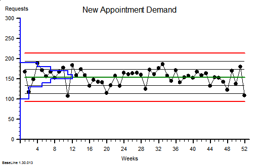
<Leslie> Yes. I recognise that. This chart shows a stable system of demand with an average of around 150 new referrals per week and the variation distributed above and below the average in a symmetrical pattern, falling off to zero around the upper and lower process limits. I believe that you said that over 99% will fall within the limits.

<Bob> Good. The blue histogram on this chart is called a probability distribution function, to use the terminology of a statistician.

<Leslie> OK.

<Bob> So, what would happen if we created a Pareto chart of demand using the number of patients per week as the categories and ignoring the time aspect? We are allowed to do that if the behaviour is stable, as this chart suggests.

<Leslie> Give me a minute, I will need to do a rough sketch. Does this look right?

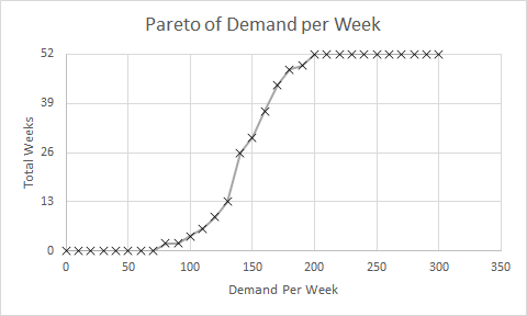
<Bob> Perfect! So if you now convert the Y-axis to a percentage scale so that 52 weeks is 100% then where does the average weekly demand of about 150 fall? Read up from the X-axis to the line then across to the Y-axis.

<Leslie> At about 26 weeks or 50% of 52 weeks. Ah ha! So that is what a percentile means! The 50th percentile is the average, the zeroth percentile is around the lower process limit and the 100th percentile is around the upper process limit!

<Bob> In this case the 50th percentile is the average, it is not always the case though. So where is the 85th percentile line?

<Leslie> Um, 52 times 0.85 is 44.2 which, reading across from the Y-axis then down to the X-axis gives a weekly demand of about 170 per week. That is about the same as the average plus one sigma according to the run chart.

<Bob> Excellent. The Pareto chart that you have drawn is called a cumulative probability distribution function … and that is usually what percentiles refer to. Comparative Statisticians love these but often omit to explain their rationale to non-statisticians!

<Leslie> Phew! So, now I can see that the 65th percentile is just above average demand, and 85th percentile is above that. But in the confusing paragraph how does that relate to the phrase “65% and 85% of the time”?

<Bob> It doesn’t. That is the really, really confusing part of that paragraph. I am not surprised that you looped out at that point!

<Leslie> OK. Let us leave that for another conversation. If I ignore that bit then does the rest of it make sense?

<Bob> Not yet alas. We need to dig a bit deeper. What would you say are the implications of this message?

<Leslie> Well. I know that if our flow-capacity is less than our average demand then we will guarantee to create an unstable queue and chaos. That is the Flaw of Averages trap.

<Bob> OK. The creator of this tool seems to know that.

<Leslie> And my outpatient manager colleagues are always complaining that they do not have enough slots to book into, so I conclude that our current flow-capacity is just above the 50th percentile.

<Bob> A reasonable hypothesis.

<Leslie> So to calm the chaos the message is saying I will need to increase my flow capacity up to the 85th percentile of demand which is from about 150 slots per week to 170 slots per week. An increase of 7% which implies a 7% increase in costs.

<Bob> Good. I am pleased that you did not fall into the intuitive trap that a increase from the 50th to the 85th percentile implies a 35/50 or 70% increase! Your estimate of 7% is a reasonable one.

<Leslie> Well it may be theoretically reasonable but it is not practically possible. We are exhorted to reduce costs by at least that amount.

<Bob> So we have a finance versus governance bun-fight with the operational managers caught in the middle: FOG. That is not the end of the litany of woes … is there anything about Did Not Attends in the model?

<Leslie> Yes indeed! We are required to enter the percentage of DNAs and what we do with them. Do we discharge them or re-book them.

<Bob> OK. Pragmatic reality is always much more interesting than academic rhetoric and this aspect of the real system rather complicates things, at least for a comparative statistician. This is where the smoke and mirrors will appear and they will be hidden inside the black magic box. To solve this conundrum we need to understand the relationship between demand, capacity, variation and yield … and it is rather counter-intuitive. So, how would you approach this problem?

<Leslie> I would use the 6M Design® framework and I would start with a map and not with a model; least of all a magic black box one that I did not design, build and verify myself.

<Bob> And how do you know that will work any better?

<Leslie> Because at the One Day ISP Workshop I saw it work with my own eyes. The queues, waits and chaos just evaporated. And it cost nothing. We already had more than enough “capacity”.

<Bob> Indeed you did. So shall we do this one as an ISP-2 project?

<Leslie> An excellent suggestion. I already feel my confidence flowing back and I am looking forward to this new challenge. Thank you again Bob.

23/01/2016

Emergent Learning

The theme this week has been emergent learning.

By that I mean the ‘ah ha’ moment that happens when lots of bits of a conceptual jigsaw go ‘click’ and fall into place.

When, what initially appears to be smoky confusion suddenly snaps into sharp clarity. Eureka! And now new learning can emerge.

This did not happen by accident. It was engineered.

The picture above is part of a bigger schematic map of a system – in this case a system related to the global health challenge of escalating obesity.

It is a complicated arrangement of boxes and arrows. There are dotted lines that outline parts of the system that have leaky boundaries like the borders on a political map.

But it is a static picture of the structure … it tells us almost nothing about the function, the system behaviour.

And our intuition tells us that, because it is a complicated structure, it will exhibit complex and difficult to understand behaviour. So, guided by our inner voice, we toss it into the pile labelled Wicked Problems and look for something easier to work on.

Our natural assumption that a complicated structure always leads to complex behavior is an invalid simplification, and one that we can disprove in a matter of moments.

Exhibit 1. A system can be complicated and yet still exhibit simple, stable and predictable behavior.

The picture is of a clock designed and built by John Harrison (1693-1776). It is called H1 and it is a sea clock.

Masters of sailing ships required very accurate clocks to calculate their longitude, the East-West coordinate on the Earth’s surface. And in the 18th Century this was a BIG problem. Too many ships were getting lost at sea.

Harrison’s sea clock is complicated. It has many moving parts, but it was the most stable and accurate clock of its time. And his later ones were smaller, more accurate and even more complicated.

Exhibit 2. A system can be simple yet still exhibit complex, unstable and unpredictable behavior.

The image is of a pendulum made of only two rods joined by a hinge. The structure is simple yet the behavior is complex, and this can only be appreciated with a dynamic visualisation.

The behaviour is clearly not random. It has an emergent structure. It is called chaotic.

So, with these two real examples we have disproved our assumption that a complicated structure always leads to complex behaviour; and we have also disproved its inverse … that complex behavior always comes from a complicated structure.

The cognitive trap we have exposed here is over-generalisation, the unconscious habit of slipping in the implied [always].

This deeper understanding gives us hope.

John Harrison was a rare, naturally-gifted, mechanical genius. And to make it easier, he was working on a purely mechanical system comprised of non-living parts that only obeyed the Laws of Newtonian physics. And even with those advantages it took him decades to learn how to design and to build his sea clocks. He was the first to do so and he was self-educated so his learning was emergent.

If there were a way to design complicated systems to exhibit stable and predictable behaviour, how could more of us learn how to do that?

Our healthcare system is not made of passive, mechanical cogs and springs. The parts are active, living people whose actions are limited by physical Laws but whose decisions are steered by other policies … learned ones … and ones that can change. These learned rules of thumb are called heuristics and they vary from person-to-person and from minute-to-minute. Heuristics can be learned, unlearned, updated, and evolved.

This is called emergent learning.

And to generate it we only need to create the context for it … the rest happens … as if by magic … but only if we design a fit-for-purpose context.

This week I personally observed over a dozen healthcare staff simultaneously re-invent a complicated process scheduling technique, at the same time as using it to eliminate the queues, waiting and chaos in the system they wanted to improve.

Their queues just evaporated … without requiring any extra capacity or money. Eureka!

We did not show them how to do it so they could not have just copied what we did.

We designed and built the context for their learning to emerge … and it did. On its own.

The One Day Practical Skills Workshop delivered emergent learning … just as it was designed to do.

A health care system is a complex adaptive system (CAS), and system improvement-by-design is what systems engineers (SE) are trained to do.

And this emerging style of complex adaptive systems engineering (CASE) is at the cutting edge of human knowledge, and when applied in the health care domain it is called health care systems engineering (HCSE).

Our experience of the emergent learning that flows from the practical skills workshops verifies that CASE is both possible, learnable, teachable, applicable and effective.

16/01/2016

Hot and Cold

Last week Bob and Leslie were exploring the data analysis trap called a two-points-in-time comparison: as illustrated by the headline “This winter has not been as bad as last … which proves that our winter action plan has worked.”

Actually it doesn’t.

But just saying that is not very helpful. We need to explain the reason why this conclusion is invalid and therefore potentially dangerous.

So here is the continuation of Bob and Leslie’s conversation.

<Bob> Hi Leslie, have you been reflecting on the two-points-in-time challenge?

<Leslie> Yes indeed, and you were correct, I did know the answer … I just didn’t know I knew if you get my drift.

<Bob> Yes, I do. So, are you willing to share your story?

<Leslie> OK, but before I do that I would like to share what happened when I described what we talked about to some colleagues. They sort of got the idea but got lost in the unfamiliar language of ‘variance’ and I realized that I needed an example to illustrate.

<Bob> Excellent … what example did you choose?

<Leslie> The UK weather – or more specifically the temperature. My reasons for choosing this were many: first it is something that everyone can relate to; secondly it has strong seasonal cycle; and thirdly because the data is readily available on the Internet.

<Bob> OK, so what specific question were you trying to answer and what data did you use?

<Leslie> The question was “Are our winters getting warmer?” and my interest in that is because many people assume that the colder the winter the more people suffer from respiratory illness and the more that go to hospital … contributing to the winter A&E and hospital pressures. The data that I used was the maximum monthly temperature from 1960 to the present recorded at our closest weather station.

<Bob> OK, and what did you do with that data?

<Leslie> Well, what I did not do was to compare this winter with last winter and draw my conclusion from that! What I did first was just to plot-the-dots … I created a time-series chart … using the BaseLine© software.

And it shows what I expected to see, a strong, regular, 12-month cycle, with peaks in the summer and troughs in the winter.

<Bob> Can you explain what the green and red lines are and why some dots are red?

<Leslie> Sure. The green line is the average for all the data. The red lines are called the upper and lower process limits. They are calculated from the data and what they say is “if the variation in this data is random then we will expect more than 99% of the points to fall between these two red lines“.

<Bob> So, we have 55 years of monthly data which is nearly 700 points which means we would expect fewer than seven to fall outside these lines … and we clearly have many more than that. For example, the winter of 1962-63 and the summer of 1976 look exceptional – a run of three consecutive dots outside the red lines. So can we conclude the variation we are seeing is not random?

<Leslie> Yes, and there is more evidence to support that conclusion. First is the reality check … I do not remember either of those exceptionally cold or hot years personally, so I asked Dr Google.

This picture from January 1963 shows copper telephone lines that are so weighed down with ice, and for so long, that they have stretched down to the ground. In this era of mobile phones we forget this was what telecommunication was like!

And just look at the young Michal Fish in the Summer of ’76! Did people really wear clothes like that?

And there is more evidence on the chart. The red dots that you mentioned are indicators that BaseLine© has detected other non-random patterns.

So the large number of red dots confirms our Mark I Eyeball conclusion … that there are signals mixed up with the noise.

<Bob> Actually, I do remember the Summer of ’76 – it was the year I did my O Levels! And your signals-in-the-noise phrase reminds me of SETI – the search for extra-terrestrial intelligence! I really enjoyed the 1997 film of Carl Sagan’s book Contact with Jodi Foster playing the role of the determined scientist who ends up taking a faster-than-light trip through space in a machine designed by ET and built by humans. And especially the line about 10 minutes from the end when those-in-high-places who had discounted her story as “unbelievable” realized they may have made an error … the line ‘Yes, that is interesting isn’t it’.

<Leslie> Ha ha! Yes. I enjoyed that film too. It had lots of great characters – her glory seeking boss; the hyper-suspicious head of national security who militarized the project; the charismatic anti-hero; the ranting radical who blew up the first alien machine; and John Hurt as her guardian angel. I must watch it again.

Anyway, back to the story. The problem we have here is that this type of time-series chart is not designed to extract the overwhelming cyclical, annual pattern so that we can search for any weaker signals … such as a smaller change in winter temperature over a longer period of time.

<Bob>Yes, that is indeed the problem with these statistical process control charts. SPC charts were designed over 60 years ago for process quality assurance in manufacturing not as a diagnostic tool in a complex adaptive system such a healthcare. So how did you solve the problem?

<Leslie> I realized that it was the regularity of the cyclical pattern that was the key. I realized that I could use that to separate out the annual cycle and to expose the weaker signals. I did that using the rational grouping feature of BaseLine© with the month-of-the-year as the group.

Now I realize why the designers of the software put this feature in! With just one mouse click the story jumped out of the screen!

<Bob> OK. So can you explain what we are looking at here?

<Leslie> Sure. This chart shows the same data as before except that I asked BaseLine© first to group the data by month and then to create a mini-chart for each month-group independently. Each group has its own average and process limits. So if we look at the pattern of the averages, the green lines, we can clearly see the annual cycle. What is very obvious now is that the process limits for each sub-group are much narrower, and that there are now very few red points … other than in the groups that are coloured red anyway … a niggle that the designers need to nail in my opinion!

<Bob> I will pass on your improvement suggestion! So are you saying that the regular annual cycle has accounted for the majority of the signal in the previous chart and that now we have extracted that signal we can look for weaker signals by looking for red flags in each monthly group?

<Leslie> Exactly so. And the groups I am most interested in are the November to March ones. So, next I filtered out the November data and plotted it as a separate chart; and I then used another cool feature of BaseLine© called limit locking.

What that means is that I have used the November maximum temperature data for the first 30 years to get the baseline average and natural process limits … and we can see that there are no red flags in that section, no obvious signals. Then I locked these limits at 1990 and this tells BaseLine© to compare the subsequent 25 years of data against these projected limits. That exposed a lot of signal flags, and we can clearly see that most of the points in the later section are above the projected average from the earlier one. This confirms that there has been a significant increase in November maximum temperature over this 55 year period.

<Bob> Excellent! You have answered part of your question. So what about December onwards?

<Leslie> I was on a roll now! I also noticed from my second chart that the December, January and February groups looked rather similar so I filtered that data out and plotted them as a separate chart.

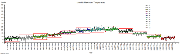
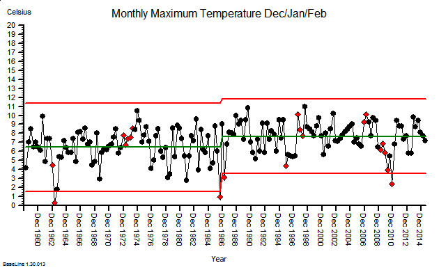
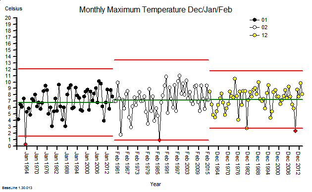
MaxTempDecJanFeb1960-2015_Grouped These were indeed almost identical so I lumped them together as a ‘winter’ group and compared the earlier half with the later half using another BaseLine© feature called segmentation.

This showed that the more recent winter months have a higher maximum temperature … on average. The difference is just over one degree Celsius. But it also shows that that the month-to-month and year-to-year variation still dominates the picture.

<Bob> Which implies?

<Leslie> That, with data like this, a two-points-in-time comparison is meaningless. If we do that we are just sampling random noise and there is no useful information in noise. Nothing that we can learn from. Nothing that we can justify a decision with. This is the reason the ‘this year was better than last year’ statement is meaningless at best; and dangerous at worst. Dangerous because if we draw an invalid conclusion, then it can lead us to make an unwise decision, then decide a counter-productive action, and then deliver an unintended outcome.

By doing invalid two-point comparisons we can too easily make the problem worse … not better.

<Bob> Yes. This is what W. Edwards Deming, an early guru of improvement science, referred to as ‘tampering‘. He was a student of Walter A. Shewhart who recognized this problem in manufacturing and, in 1924, invented the first control chart to highlight it, and so prevent it. My grandmother used the term meddling to describe this same behavior … and I now use that term as one of the eight sources of variation. Well done Leslie!

09/01/2016

The Two-Points-In-Time Comparison Trap

[Bzzzzzz] Bob’s phone vibrated to remind him it was time for the regular ISP remote coaching session with Leslie. He flipped the lid of his laptop just as Leslie joined the virtual meeting.

<Leslie> Hi Bob, and Happy New Year!

<Bob> Hello Leslie and I wish you well in 2016 too. So, what shall we talk about today?

<Leslie> Well, given the time of year I suppose it should be the Winter Crisis. The regularly repeating annual winter crisis. The one that feels more like the perpetual winter crisis.

<Bob> OK. What specifically would you like to explore?

<Leslie> Specifically? The habit of comparing of this year with last year to answer the burning question “Are we doing better, the same or worse?” Especially given the enormous effort and political attention that has been focused on the hot potato of A&E 4-hour performance.

<Bob> Aaaaah! That old chestnut! Two-Points-In-Time comparison.

<Leslie> Yes. I seem to recall you usually add the word ‘meaningless’ to that phrase.

<Bob> H’mm. Yes. It can certainly become that, but there is a perfectly good reason why we do this.

<Leslie> Indeed, it is because we see seasonal cycles in the data so we only want to compare the same parts of the seasonal cycle with each other. The apples and oranges thing.

<Bob> Yes, that is part of it. So what do you feel is the problem?

<Leslie> It feels like a lottery! It feels like whether we appear to be better or worse is just the outcome of a random toss.

<Bob> Ah! So we are back to the question “Is the variation I am looking at signal or noise?”

<Leslie> Yes, exactly.

<Bob> And we need a scientifically robust way to answer it. One that we can all trust.

<Leslie> Yes.

<Bob> So how do you decide that now in your improvement work? How do you do it when you have data that does not show a seasonal cycle?

<Leslie> I plot-the-dots and use an XmR chart to alert me to the presence of the signals I am interested in – especially a change of the mean.

<Bob> Good. So why can we not use that approach here?

<Leslie> Because the seasonal cycle is usually a big signal and it can swamp the smaller change I am looking for.

<Bob> Exactly so. Which is why we have to abandon the XmR chart and fall back the two points in time comparison?

<Leslie> That is what I see. That is the argument I am presented with and I have no answer.

<Bob> OK. It is important to appreciate that the XmR chart was not designed for doing this. It was designed for monitoring the output quality of a stable and capable process. It was designed to look for early warning signs; small but significant signals that suggest future problems. The purpose is to alert us so that we can identify the root causes, correct them and the avoid a future problem.

<Leslie> So we are using the wrong tool for the job. I sort of knew that. But surely there must be a better way than a two-points-in-time comparison!

<Bob> There is, but first we need to understand why a TPIT is a poor design.

<Leslie> Excellent. I’m all ears.

<Bob> A two point comparison is looking at the difference between two values, and that difference can be positive, zero or negative. In fact, it is very unlikely to be zero because noise is always present.

<Leslie> OK.

<Bob> Now, both of the values we are comparing are single samples from two bigger pools of data. It is the difference between the pools that we are interested in but we only have single samples of each one … so they are not measurements … they are estimates.

<Leslie> So, when we do a TPIT comparison we are looking at the difference between two samples that come from two pools that have inherent variation and may or may not actually be different.

<Bob> Well put. We give that inherent variation a name … we call it variance … and we can quantify it.

<Leslie> So if we do many TPIT comparisons then they will show variation as well … for two reasons; first because the pools we are sampling have inherent variation; and second just from the process of sampling itself. It was the first lesson in the ISP-1 course.

<Bob> Well done! So the question is: “How does the variance of the TPIT sample compare with the variance of the pools that the samples are taken from?”

<Leslie> My intuition tells me that it will be less because we are subtracting.

<Bob> Your intuition is half-right. The effect of the variation caused by the signal will be less … that is the rationale for the TPIT after all … but the same does not hold for the noise.

<Leslie> So the noise variation in the TPIT is the same?

<Bob> No. It is increased.

<Leslie> What! But that would imply that when we do this we are less likely to be able to detect a change because a small shift in signal will be swamped by the increase in the noise!

<Bob> Precisely. And the degree that the variance increases by is mathematically predictable … it is increased by a factor of two.

<Leslie> So as we usually present variation as the square root of the variance, to get it into the same units as the metric, then that will be increased by the square root of two … 1.414

<Bob> Yes.

<Leslie> I need to put this counter-intuitive theory to the test!

<Bob> Excellent. Accept nothing on faith. Always test assumptions. And how will you do that?

<Leslie> I will use Excel to generate a big series of normally distributed random numbers; then I will calculate a series of TPIT differences using a fixed time interval; then I will calculate the means and variations of the two sets of data; and then I will compare them.

<Bob> Excellent. Let us reconvene in ten minutes when you have done that.

10 minutes later …

<Leslie> Hi Bob, OK I am ready and I would like to present the results as charts. Is that OK?

<Bob> Perfect!

<Leslie> Here is the first one. I used our A&E performance data to give me some context. We know that on Mondays we have an average of 210 arrivals with an approximately normal distribution and a standard deviation of 44; so I used these values to generate the random numbers. Here is the simulated Monday Arrivals chart for two years.

<Bob> OK. It looks stable as we would expect and I see that you have plotted the sigma levels which look to be just under 50 wide.

<Leslie> Yes, it shows that my simulation is working. So next is the chart of the comparison of arrivals for each Monday in Year 2 compared with the corresponding week in Year 1.

<Bob> Oooookaaaaay. What have we here? Another stable chart with a mean of about zero. That is what we would expect given that there has not been a change in the average from Year 1 to Year 2. And the variation has increased … sigma looks to be just over 60.

<Leslie> Yes! Just as the theory predicted. And this is not a spurious answer. I ran the simulation dozens of times and the effect is consistent! So, I am forced by reality to accept the conclusion that when we do two-point-in-time comparisons to eliminate a cyclical signal we will reduce the sensitivity of our test and make it harder to detect other signals.

<Bob> Good work Leslie! Now that you have demonstrated this to yourself using a carefully designed and conducted simulation experiment, you will be better able to explain it to others.

<Leslie> So how do we avoid this problem?

<Bob> An excellent question and one that I will ask you to ponder on until our next chat. You know the answer to this … you just need to bring it to conscious awareness.