Spring the Trap

trapped_in_question_PA_300_wht_3174[Beeeeeep] It was time for the weekly coaching chat.  Bob, a seasoned practitioner of flow science, dialled into the teleconference with Lesley.

<Bob> Good afternoon Lesley, can I suggest a topic today?

<Lesley> Hi Bob. That would be great, and I am sure you have a good reason for suggesting it.

<Bob> I would like to explore the concept of time-traps again because it something that many find confusing. Which is a shame because it is often the key to delivering surprisingly dramatic and rapid improvements; at no cost.

<Lesley> Well doing exactly that is what everyone seems to be clamouring for so it sounds like a good topic to me.  I confess that I am still not confident to teach others about time-traps.

<Bob> OK. Let us start there. Can you describe what happens when you try to teach it?

<Lesley> Well, it seems to be when I say that the essence of a time-trap is that the lead time and the flow are independent.  For example, the lead time stays the same even though the flow is changing.  That really seems to confuse people; and me too if I am brutally honest.

<Bob> OK.  Can you share the example that you use?

<Lesley> Well it depends on who I am talking to.  I prefer to use an example that they are familiar with.  If it is a doctor I might use the example of the ward round.  If it is a manager I might use the example of emails or meetings.

<Bob> Assume I am a doctor then – an urgent care physician.

<Lesley> OK.  Let us take it that I have done the 4N Chart and the  top niggle is ‘Frustration because the post-take ward round takes so long that it delays the discharge of patients who then often have to stay an extra night which then fills up the unit with waiting patients and we get blamed for blocking flow from A&E and causing A&E breaches‘.

<Bob> That sounds like a good example. What is the time-trap in that design?

<Lesley> The  post-take ward round.

<Bob> And what justification is usually offered for using that design?

<Lesley> That it is a more efficient use of the expensive doctor’s time if the whole team congregate once a day and work through all the patients admitted over the previous 24 hours.  They review the presentation, results of tests, diagnosis, management plans, response to treatment, decide the next steps and do the paperwork.

<Bob> And why is that a time-trap design?

<Lesley> Because  it does not matter if one patient is admitted or ten, the average lead time from the perspective of the patient is the same – about one day.

<Bob> Correct. So why is the doctor complaining that there are always lots of patients to see?

<Lesley> Because there are. The emergency short stay ward is usually full by the time the post take ward round happens.

<Bob> And how do you present the data that shows the lead time is independent of the flow?

<Lesley> I use a Gantt chart, but the problem I find is that there is so much variation and queue jumping it is not blindingly obvious from the Gantt chart that there is a time-trap. There is so much else clouding the picture.

<Bob>Is that where the ‘but I do not understand‘ conversation starts?

<Lesley> Yes. And that is where I get stuck too.

<Bob> OK.  The issue here is that a Gantt chart is not the ideal visualisation tool when there are lots of crossed-streams, frequently changing priorities, and many other sources of variation.  The Gantt chart gets ‘messy’.   The trick here is to use a Vitals Chart – and you can derive that from the same data you used for the Gantt chart.

<Lesley> You are right about the Gantt chart getting messy. I have seen massive wall-sized Gantt charts that are veritable works-of-art and that have taken hours to create; and everyone standing looking at it and saying ‘Wow! That is an impressive piece of work.  So what does it tell us? How does it help?

<Bob> Yes, I have experienced that too. I think what happens is that those who do the foundation training and discover the Gantt chart then try to use it to solve every flow problem – and in their enthusiasm they discount any warning advice.  Desperation drives over-inflated expectation which is often the pre-cursor to disappointment, and then disillusionment.  The Nerve Curve again.

<Lesley> But a Vitals Chart is an HCSE level technique and you said that we do not need to put everyone through HCSE training.

<Bob>That is correct. I am advocating an HCSE-in-training using a Vitals Chart to explain the concept of a time-trap so that everyone understands it well enough to see the flaw in the design.

<Lesley> Ah ha!  Yes, I see.  So what is my next step?

<Bob> I will let you answer that.

<Lesley> Um, let me think.

The outcome I want is everyone understands the concept of a time-trap well enough to feel comfortable with trying a time-trap-free design because they can see the benefits for them.

And to get that depth of understanding I need to design a table top exercise that starts with a time-trap design and generates raw data that we can use to build both a Gantt chart and the Vitals Chart; so I can point out and explain the characteristic finger-print of a time trap.

And then we can ‘test’ an alternative time-trap-free design and generate the prognostic Gantt and Vitals Chart and compare with the baseline diagnostic charts to reveal the improvement.

<Bob> That sounds like a good plan to me.  And if you do that, and your team apply it to a real improvement exercise, and you see the improvement and you share the story, then that will earn you a coveted HCSE Certificate of Competency.

<Lesley>Ah ha! Now I understand the reason you suggested this topic!  I am on the case!

The Time Trap

clock_hands_spinning_import_150_wht_3149[Hmmmmmm] The desk amplified the vibration of Bob’s smartphone as it signaled the time for his planned e-mentoring session with Leslie.

[Dring Dring]

<Bob> Hi Leslie, right-on-time, how are you today?

<Leslie> Good thanks Bob. I have a specific topic to explore if that is OK. Can we talk about time traps.

<Bob> OK – do you have a specific reason for choosing that topic?

<Leslie> Yes. The blog last week about ‘Recipe for Chaos‘ set me thinking and I remembered that time-traps were mentioned in the FISH course but I confess, at the time, I did not understand them. I still do not.

<Bob> Can you describe how the ‘Recipe for Chaos‘ blog triggered this renewed interest in time-traps?

<Leslie> Yes – the question that occurred to me was: ‘Is a time-trap a recipe for chaos?’

<Bob> A very good question! What do you feel the answer is?

<Leslie>I feel that time-traps can and do trigger chaos but I cannot explain how. I feel confused.

<Bob>Your intuition is spot on – so can you localize the source of your confusion?

<Leslie>OK. I will try. I confess I got the answer to the MCQ correct by guessing – and I wrote down the answer when I eventually guessed correctly – but I did not understand it.

<Bob>What did you write down?

<Leslie>“The lead time is independent of the flow”.

<Bob>OK. That is accurate – though I agree it is perhaps a bit abstract. One source of confusion may be that there are different causes of of time-traps and there is a lot of overlap with other chaos-creating policies. Do you have a specific example we can use to connect theory with reality?

<Leslie> OK – that might explain my confusion.  The example that jumped to mind is the RTT target.

<Bob> RTT?

<Leslie> Oops – sorry – I know I should not use undefined abbreviations. Referral to Treatment Time.

<Bob> OK – can you describe what you have mapped and measured already?

<Leslie> Yes.  When I plot the lead-time for patients in date-of-treatment order the process looks stable but the histogram is multi-modal with a big spike just underneath the RTT target of 18 weeks. What you describe as the ‘Horned Gaussian’ – the sign that the performance target is distorting the behaviour of the system and the design of the system is not capable on its own.

<Bob> OK and have you investigated why there is not just one spike?

<Leslie> Yes – the factor that best explains that is the ‘priority’ of the referral.  The  ‘urgents’ jump in front of the ‘soons’ and both jump in front of the ‘routines’. The chart has three overlapping spikes.

<Bob> That sounds like a reasonable policy for mixed-priority demand. So what is the problem?

<Leslie> The ‘Routine’ group is the one that clusters just underneath the target. The lead time for routines is almost constant but most of the time those patients sit in one queue or another being leap-frogged by other higher-priority patients. Until they become high-priority – then they do the leap frogging.

<Bob> OK – and what is the condition for a time trap again?

<Leslie> That the lead time is independent of flow.

<Bob>Which implies?

<Leslie> Um. let me think. That the flow can be varying but the lead time stays the same?

<Bob> Yup. So is the flow of routine referrals varying?

<Leslie> Not over the long term. The chart is stable.

<Bob> What about over the short term? Is demand constant?

<Leslie>No of course not – it varies – but that is expected for all systems. Constant means ‘over-smoothed data’ – the Flaw of Averages trap!

<Bob>OK. And how close is the average lead time for routines to the RTT maximum allowable target?

<Leslie> Ah! I see what you mean. The average is about 17 weeks and the target is 18 weeks.

<Bob>So what is the flow variation on a week-to-week time scale?

<Leslie>Demand or Activity?

<Bob>Both.

<Leslie>H’mm – give me a minute to re-plot flow as a weekly-aggregated chart. Oh! I see what you mean – both the weekly activity and demand are both varying widely and they are not in sync with each other. Work in progress must be wobbling up and down a lot! So how can the lead time variation be so low?

<Bob>What do the flow histograms look like?

<Leslie> Um. Just a second. That is weird! They are both bi-modal with peaks at the extremes and not much in the middle – the exact opposite of what I expected to see! I expected a centered peak.

<Bob>What you are looking at is the characteristic flow fingerprint of a chaotic system – it is called ‘thrashing’.

<Leslie> So I was right!

<Bob> Yes. And now you know the characteristic pattern to look for. So what is the policy design flaw here?

<Leslie>The DRAT – the delusional ratio and arbitrary target?

<Bob> That is part of it – that is the external driver policy. The one you cannot change easily. What is the internally driven policy? The reaction to the DRAT?

<Leslie> The policy of leaving routine patients until they are about to breach then re-classifying them as ‘urgent’.

<Bob>Yes! It is called a ‘Prevarication Policy’ and it is surprisingly and uncomfortably common. Ask yourself – do you ever prevaricate? Do you ever put off ‘lower priority’ tasks until later and then not fill the time freed up with ‘higher priority tasks’?

<Leslie> OMG! I do that all the time! I put low priority and unexciting jobs on a ‘to do later’ heap but I do not sit idle – I do then focus on the high priority ones.

<Bob> High priority for whom?

<Leslie> Ah! I see what you mean. High priority for me. The ones that give me the biggest reward! The fun stuff or the stuff that I get a pat on the back for doing or that I feel good about.

<Bob> And what happens?

<Leslie> The heap of ‘no-fun-for-me-to-do’ jobs gets bigger and I await the ‘reminders’ and then have to rush round in a mad panic to avoid disappointment, criticism and blame. It feels chaotic. I get grumpy. I make more mistakes and I deliver lower-quality work. If I do not get a reminder I assume that the job was not that urgent after all and if I am challenged I claim I am too busy doing the other stuff.

<Bob> Have you avoided disappointment?

<Leslie> Ah! No – that I needed to be reminded meant that I had already disappointed. And when I do not get a reminded does not prove I have not disappointed either. Most people blame rather than complain. I have just managed to erode other people’s trust in my reliability. I have disappointed myself. I have achieved exactly the opposite of what I intended. Drat!

<Bob> So what is the reason that you work this way? There will be a reason.  A good reason.

<Leslie> That is a very good question! I will reflect on that because I believe it will help me understand why others behave this way too.

<Bob> OK – I will be interested to hear your conclusion.  Let us return to the question. What is the  downside of a ‘Prevarication Policy’?

<Leslie> It creates stress, chaos, fire-fighting, last minute changes, increased risk of errors,  more work and it erodes both quality, confidence and trust.

<Bob>Indeed so – and the impact on productivity?

<Leslie> The activity falls, the system productivity falls, revenue falls, queues increase, waiting times increase and the chaos increases!

<Bob> And?

<Leslie> We treat the symptoms by throwing resources at the problem – waiting list initiatives – and that pushes our costs up. Either way we are heading into a spiral of decline and disappointment. We do not address the root cause.

<Bob> So what is the way out of chaos?

<Leslie> Reduce the volume on the destabilizing feedback loop? Stop the managers meddling!

<Bob> Or?

<Leslie> Eh? I do not understand what you mean. The blog last week said management meddling was the problem.

<Bob> It is a problem. How many feedback loops are there?

<Leslie> Two – that need to be balanced.

<Bob> So what is another option?

<Leslie> OMG! I see. Turn UP the volume of the stabilizing feedback loop!

<Bob> Yup. And that is a lot easier to do in reality. So that is your other challenge to reflect on this week. And I am delighted to hear you using the terms ‘stabilizing feedback loop’ and ‘destabilizing feedback loop’.

<Leslie> Thank you. That was a lesson for me after last week – when I used the terms ‘positive and negative feedback’ it was interpreted in the emotional context – positive feedback as encouragement and negative feedback as criticism.  So ‘reducing positive feedback’ in that sense is the exact opposite of what I was intending. So I switched my language to using ‘stabilizing and destabilizing’ feedback loops that are much less ambiguous and the confusion and conflict disappeared.

<Bob> That is very useful learning Leslie … I think I need to emphasize that distinction more in the blog. That is one advantage of online media – it can be updated!

 <Leslie> Thanks again Bob!  And I have the perfect opportunity to test a new no-prevarication-policy design – in part of the system that I have complete control over – me!

The Recipe for Chaos

boxes_group_PA4_150_wht_4916There are only four ingredients required to create Chaos.

The first is Time.

All processes and systems are time-dependent.

The second ingredient is a Metric of Interest (MoI).

That means a system performance metric that is important to all – such as a Safety or Quality or Cost; and usually all three.

The third ingredient is a feedback loop of a specific type – it is called a Negative Feedback Loop.  The NFL  is one that tends to adjust, correct and stabilise the behaviour of the system.

Negative feedback loops are very useful – but they have a drawback. They resist change and they reduce agility. The name is also a disadvantage – the word ‘negative feedback’ is often associated with criticism.

The fourth and final ingredient in our Recipe for Chaos is also a feedback loop but one of a different design – a Positive Feedback Loop (PFL)- one that amplifies variation and change.

Positive feedback loops are also very useful – they are required for agility – quick reactions to unexpected events. Fast reflexes.

The downside of a positive feedback loop is that increases instability.

The name is also confusing – ‘positive feedback’ is associated with encouragement and praise.

So, in this context it is better to use the terms ‘stabilizing feedback’ and ‘destabilizing feedback’  loops.

When we mix these four ingredients in just the right amounts we get a system that may behave chaotically. That is surprising and counter-intuitive. But it is how the Universe works.

For example:

Suppose our Metric of Interest is the amount of time that patients spend in a Accident and Emergency Department. We know that the longer this time is the less happy they are and the higher the risk of avoidable harm – so it is a reasonable goal to reduce it.

Longer-than-possible waiting times have many root causes – it is a non-specific metric.  That means there are many things that could be done to reduce waiting time and the most effective actions will vary from case-to-case, day-to-day and even minute-to-minute.  There is no one-size-fits-all solution.

This implies that those best placed to correct the causes of these delays are the people who know the specific system well – because they work in it. Those who actually deliver urgent care. They are the stabilizing ingredient in our Recipe for Chaos.

The destabilizing ingredient is the hit-the-arbitrary-target policy which drives a performance management feedback loop.

This policy typically involves:
(1) Setting a performance target that is desirable but impossible for the current design to achieve reliably;
(2) inspecting how close to the target we are; then
(3) using the real-time data to justify threats of dire consequences for failure.

Now we have a perfect Recipe for Chaos.

The higher the failure rate the more inspections, reports, meetings, exhortations, threats, interruptions, and interventions that are generated.  Fear-fuelled management meddling. This behaviour consumes valuable time – so leaves less time to do the worthwhile work. Less time to devote to safety, flow, and quality. The queues build and the pressure increases and the system becomes hyper-sensitive to small fluctuations. Delays multiply and errors are more likely and spawn more workload, more delays and more errors.  Tempers become frayed and molehills are magnified into mountains. Irritations become arguments.  And all of this makes the problem worse rather than better. Less stable. More variable. More chaotic. More dangerous. More expensive.

It is actually possible to write a simple equation that captures this complex dynamic behaviour characteristic of real systems.  And that was a very surprising finding when it was discovered in 1976 by a mathematician called Robert May.

This equation is called the logistic equation.

Here is the abstract of his seminal paper.

Nature 261, 459-467 (10 June 1976)

Simple mathematical models with very complicated dynamics

First-order difference equations arise in many contexts in the biological, economic and social sciences. Such equations, even though simple and deterministic, can exhibit a surprising array of dynamical behaviour, from stable points, to a bifurcating hierarchy of stable cycles, to apparently random fluctuations. There are consequently many fascinating problems, some concerned with delicate mathematical aspects of the fine structure of the trajectories, and some concerned with the practical implications and applications. This is an interpretive review of them.

The fact that this chaotic behaviour is completely predictable and does not need any ‘random’ element was a big surprise. Chaotic is not the same as random. The observed chaos in the urgent healthcare care system is the result of the design of the system – or more specifically the current healthcare system management policies.

This has a number of profound implications – the most important of which is this:

If the chaos we observe in our health care systems is the predictable and inevitable result of the management policies we ourselves have created and adopted – then eliminating the chaos will only require us to re-design these policies.

In fact we only need to tweak one of the ingredients of the Recipe for Chaos – such as to reduce the strength of the destabilizing feedback loop. The gain. The volume control on the variation amplifier!

This is called the MM factor – otherwise known as ‘Management Meddling‘.

We need to keep all four ingredients though – because we need our system to have both agility and stability.  It is the balance of ingredients that that is critical.

The flaw is not the Managers themselves – it is their learned behaviour – the Meddling.  This is learned so it can be unlearned. We need to keep the Managers but “tweak” their role slightly. As they unlearn their old habits they move from being ‘Policy-Enforcers and Fire-Fighters’ to becoming ‘Policy-Engineers and Chaos-Calmers’. They focus on learning to understand the root causes of variation that come from outside the circle of influence of the non-Managers.   They learn how to rationally and radically redesign system policies to achieve both agility and stability.

And doing that requires developing systemic-thinking and learning Improvement Science skills – because the causes of chaos are counter-intuitive. If it were intuitively-obvious we would have discovered the nature of chaos thousands of years ago. The fact that it was not discovered until 1976 demonstrates this fact.

It is our homo sapiens intuition that got us into this mess!  The inherent flaws of the chimp-ware between our ears.  Our current management policies are intuitively-obvious, collectively-agreed, rubber-stamped and wrong! They are part of the Recipe for Chaos.

And when we learn to re-design our system policies and upload the new system software then the chaos evaporates as if a magic wand had been waved.

And that comes as a really BIG surprise!

What also comes as a big surprise is just how small the counter-intuitive policy design tweaks often are.

Safe, smooth, efficient, effective, and productive flow is restored. Calm confidence reigns. Safety, Flow, Quality and Productivity all increase – at the same time.  The emotional storm clouds dissipate and the prosperity sun shines again.

Everyone feels better. Everyone. Patients, managers, and non-managers.

This is Win-Win-Win improvement by design. Improvement Science.

Look Out For The Time Trap!

There is a common system ailment which every Improvement Scientist needs to know how to manage.

In fact, it is probably the commonest.

The Symptoms: Disappointingly long waiting times and all resources running flat out.

The Diagnosis?  90%+ of managers say “It is obvious – lack of capacity!”.

The Treatment? 90%+ of managers say “It is obvious – more capacity!!”

Intuitively obvious maybe – but unfortunately these are incorrect answers. Which implies that 90%+ of managers do not understand how their systems work. That is a bit of a worry.  Lament not though – misunderstanding is a treatable symptom of an endemic system disease called agnosia (=not knowing).

The correct answer is “I do not yet have enough information to make a diagnosis“.

This answer is more helpful than it looks because it prompts four other questions:

Q1. “What other possible system diagnoses are there that could cause this pattern of symptoms?”
Q2. “What do I need to know to distinguish these system diagnoses?”
Q3. “How would I treat the different ones?”
Q4. “What is the risk of making the wrong system diagnosis and applying the wrong treatment?”


Before we start on this list we need to set out a few ground rules that will protect us from more intuitive errors (see last week).

The first Rule is this:

Rule #1: Data without context is meaningless.

For example 130  is a number – it is data. 130 what? 130 mmHg. Ah ha! The “mmHg” is the units – it means millimetres of mercury and it tells us this data is a pressure. But what, where, when,who, how and why? We need more context.

“The systolic blood pressure measured in the left arm of Joe Bloggs, a 52 year old male, using an Omron M2 oscillometric manometer on Saturday 20th October 2012 at 09:00 is 130 mmHg”.

The extra context makes the data much more informative. The data has become information.

To understand what the information actually means requires some prior knowledge. We need to know what “systolic” means and what an “oscillometric manometer” is and the relevance of the “52 year old male”.  This ability to extract meaning from information has two parts – the ability to recognise the language – the syntax; and the ability to understand the concepts that the words are just labels for; the semantics.

To use this deeper understanding to make a wise decision to do something (or not) requires something else. Exploring that would  distract us from our current purpose. The point is made.

Rule #1: Data without context is meaningless.

In fact it is worse than meaningless – it is dangerous. And it is dangerous because when the context is missing we rarely stop and ask for it – we rush ahead and fill the context gaps with assumptions. We fill the context gaps with beliefs, prejudices, gossip, intuitive leaps, and sometimes even plain guesses.

This is dangerous – because the same data in a different context may have a completely different meaning.

To illustrate.  If we change one word in the context – if we change “systolic” to “diastolic” then the whole meaning changes from one of likely normality that probably needs no action; to one of serious abnormality that definitely does.  If we missed that critical word out then we are in danger of assuming that the data is systolic blood pressure – because that is the most likely given the number.  And we run the risk of missing a common, potentially fatal and completely treatable disease called Stage 2 hypertension.

There is a second rule that we must always apply when using data from systems. It is this:

Rule #2: Plot time-series data as a chart – a system behaviour chart (SBC).

The reason for the second rule is because the first question we always ask about any system must be “Is our system stable?”

Q: What do we mean by the word “stable”? What is the concept that this word is a label for?

A: Stable means predictable-within-limits.

Q: What limits?

A: The limits of natural variation over time.

Q: What does that mean?

A: Let me show you.

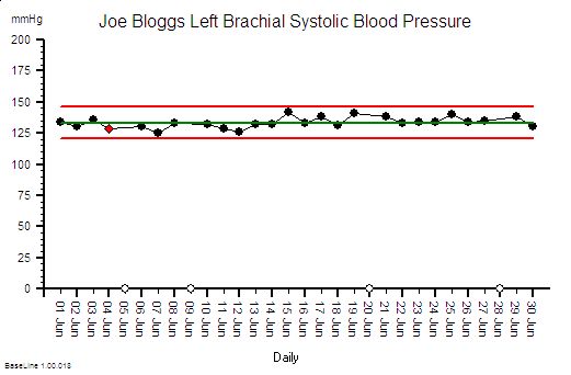
Joe Bloggs is disciplined. He measures his blood pressure almost every day and he plots the data on a chart together with some context .  The chart shows that his systolic blood pressure is stable. That does not mean that it is constant – it does vary from day to day. But over time a pattern emerges from which Joe Bloggs can see that, based on past behaviour, there is a range within which future behaviour is predicted to fall.  And Joe Bloggs has drawn these limits on his chart as two red lines and he has called them expectation lines. These are the limits of natural variation over time of his systolic blood pressure.

If one day he measured his blood pressure and it fell outside that expectation range  then he would say “I didn’t expect that!” and he could investigate further. Perhaps he made an error in the measurement? Perhaps something else has changed that could explain the unexpected result. Perhaps it is higher than expected because he is under a lot of emotional stress a work? Perhaps it is lower than expected because he is relaxing on holiday?

His chart does not tell him the cause – it just flags when to ask more “What might have caused that?” questions.

If you arrive at a hospital in an ambulance as an emergency then the first two questions the emergency care team will need to know the answer to are “How sick are you?” and “How stable are you?”. If you are sick and getting sicker then the first task is to stabilise you, and that process is called resuscitation.  There is no time to waste.


So how is all this relevant to the common pattern of symptoms from our sick system: disappointingly long waiting times and resources running flat out?

Using Rule#1 and Rule#2:  To start to establish the diagnosis we need to add the context to the data and then plot our waiting time information as a time series chart and ask the “Is our system stable?” question.

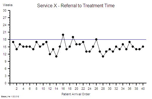
Suppose we do that and this is what we see. The context is that we are measuring the Referral-to-Treatment Time (RTT) for consecutive patients referred to a single service called X. We only know the actual RTT when the treatment happens and we want to be able to set the expectation for new patients when they are referred  – because we know that if patients know what to expect then they are less likely to be disappointed – so we plot our retrospective RTT information in the order of referral.  With the Mark I Eyeball Test (i.e. look at the chart) we form the subjective impression that our system is stable. It is delivering a predictable-within-limits RTT with an average of about 15 weeks and an expected range of about 10 to 20 weeks.

So far so good.

Unfortunately, the purchaser of our service has set a maximum limit for RTT of 18 weeks – a key performance indicator (KPI) target – and they have decided to “motivate” us by withholding payment for every patient that we do not deliver on time. We can now see from our chart that failures to meet the RTT target are expected, so to avoid the inevitable loss of income we have to come up with an improvement plan. Our jobs will depend on it!

Now we have a problem – because when we look at the resources that are delivering the service they are running flat out – 100% utilisation. They have no spare flow-capacity to do the extra work needed to reduce the waiting list. Efficiency drives and exhortation have got us this far but cannot take us any further. We conclude that our only option is “more capacity”. But we cannot afford it because we are operating very close to the edge. We are a not-for-profit organisation. The budgets are tight as a tick. Every penny is being spent. So spending more here will mean spending less somewhere else. And that will cause a big argument.

So the only obvious option left to us is to change the system – and the easiest thing to do is to monitor the waiting time closely on a patient-by-patient basis and if any patient starts to get close to the RTT Target then we bump them up the list so that they get priority. Obvious!

WARNING: We are now treating the symptoms before we have diagnosed the underlying disease!

In medicine that is a dangerous strategy.  Symptoms are often not-specific.  Different diseases can cause the same symptoms.  An early morning headache can be caused by a hangover after a long night on the town – it can also (much less commonly) be caused by a brain tumour. The risks are different and the treatment is different. Get that diagnosis wrong and disappointment will follow.  Do I need a hole in the head or will a paracetamol be enough?


Back to our list of questions.

What else can cause the same pattern of symptoms of a stable and disappointingly long waiting time and resources running at 100% utilisation?

There are several other process diseases that cause this symptom pattern and none of them are caused by lack of capacity.

Which is annoying because it challenges our assumption that this pattern is always caused by lack of capacity. Yes – that can sometimes be the cause – but not always.

But before we explore what these other system diseases are we need to understand why our current belief is so entrenched.

One reason is because we have learned, from experience, that if we throw flow-capacity at the problem then the waiting time will come down. When we do “waiting list initiatives” for example.  So if adding flow-capacity reduces the waiting time then the cause must be lack of capacity? Intuitively obvious.

Intuitively obvious it may be – but incorrect too.  We have been tricked again. This is flawed causal logic. It is called the illusion of causality.

To illustrate. If a patient complains of a headache and we give them paracetamol then the headache will usually get better.  That does not mean that the cause of headaches is a paracetamol deficiency.  The headache could be caused by lots of things and the response to treatment does not reliably tell us which possible cause is the actual cause. And by suppressing the symptoms we run the risk of missing the actual diagnosis while at the same time deluding ourselves that we are doing a good job.

If a system complains of  long waiting times and we add flow-capacity then the long waiting time will usually get better. That does not mean that the cause of long waiting time is lack of flow-capacity.  The long waiting time could be caused by lots of things. The response to treatment does not reliably tell us which possible cause is the actual cause – so by suppressing the symptoms we run the risk of missing the diagnosis while at the same time deluding ourselves that we are doing a good job.

The similarity is not a co-incidence. All systems behave in similar ways. Similar counter-intuitive ways.


So what other system diseases can cause a stable and disappointingly long waiting time and high resource utilisation?

The commonest system disease that is associated with these symptoms is a time trap – and they have nothing to do with capacity or flow.

They are part of the operational policy design of the system. And we actually design time traps into our systems deliberately! Oops!

We create a time trap when we deliberately delay doing something that we could do immediately – perhaps to give the impression that we are very busy or even overworked!  We create a time trap whenever we deferring until later something we could do today.

If the task does not seem important or urgent for us then it is a candidate for delaying with a time trap.

Unfortunately it may be very important and urgent for someone else – and a delay could be expensive for them.

Creating time traps gives us a sense of power – and it is for that reason they are much loved by bureaucrats.

To illustrate how time traps cause these symptoms consider the following scenario:

Suppose I have just enough resource-capacity to keep up with demand and flow is smooth and fault-free.  My resources are 100% utilised;  the flow-in equals the flow-out; and my waiting time is stable.  If I then add a time trap to my design then the waiting time will increase but over the long term nothing else will change: the flow-in,  the flow-out,  the resource-capacity, the cost and the utilisation of the resources will all remain stable.  I have increased waiting time without adding or removing capacity. So lack of resource-capacity is not always the cause of a longer waiting time.

This new insight creates a new problem; a BIG problem.

Suppose we are measuring flow-in (demand) and flow-out (activity) and time from-start-to-finish (lead time) and the resource usage (utilisation) and we are obeying Rule#1 and Rule#2 and plotting our data with its context as system behaviour charts.  If we have a time trap in our system then none of these charts will tell us that a time-trap is the cause of a longer-than-necessary lead time.

Aw Shucks!

And that is the primary reason why most systems are infested with time traps. The commonly reported performance metrics we use do not tell us that they are there.  We cannot improve what we cannot see.

Well actually the system behaviour charts do hold the clues we need – but we need to understand how systems work in order to know how to use the charts to make the time trap diagnosis.

Q: Why bother though?

A: Simple. It costs nothing to remove a time trap.  We just design it out of the process. Our flow-in will stay the same; our flow-out will stay the same; the capacity we need will stay the same; the cost will stay the same; the revenue will stay the same but the lead-time will fall.

Q: So how does that help me reduce my costs? That is what I’m being nailed to the floor with as well!

A: If a second process requires the output of the process that has a hidden time trap then the cost of the queue in the second process is the indirect cost of the time trap.  This is why time traps are such a fertile cause of excess cost – because they are hidden and because their impact is felt in a different part of the system – and usually in a different budget.

To illustrate. Suppose that 60 patients per day are discharged from our hospital and each one requires a prescription of to-take-out (TTO) medications to be completed before they can leave.  Suppose that there is a time trap in this drug dispensing and delivery process. The time trap is a policy where a porter is scheduled to collect and distribute all the prescriptions at 5 pm. The porter is busy for the whole day and this policy ensures that all the prescriptions for the day are ready before the porter arrives at 5 pm.  Suppose we get the event data from our electronic prescribing system (EPS) and we plot it as a system behaviour chart and it shows most of the sixty prescriptions are generated over a four hour period between 11 am and 3 pm. These prescriptions are delivered on paper (by our busy porter) and the pharmacy guarantees to complete each one within two hours of receipt although most take less than 30 minutes to complete. What is the cost of this one-delivery-per-day-porter-policy time trap? Suppose our hospital has 500 beds and the total annual expense is £182 million – that is £0.5 million per day.  So sixty patients are waiting for between 2 and 5 hours longer than necessary, because of the porter-policy-time-trap, and this adds up to about 5 bed-days per day – that is the cost of 5 beds – 1% of the total cost – about £1.8 million.  So the time trap is, indirectly, costing us the equivalent of £1.8 million per annum.  It would be much more cost-effective for the system to have a dedicated porter working from 12 am to 5 pm doing nothing else but delivering dispensed TTOs as soon as they are ready!  And assuming that there are no other time traps in the decision-to-discharge process;  such as the time trap created by batching all the TTO prescriptions to the end of the morning ward round; and the time trap created by the batch of delivered TTOs waiting for the nurses to distribute them to the queue of waiting patients!


Q: So how do we nail the diagnosis of a time trap and how do we differentiate it from a Batch or a Bottleneck or Carveout?

A: To learn how to do that will require a bit more explanation of the physics of processes.

And anyway if I just told you the answer you would know how but might not understand why it is the answer. Knowledge and understanding are not the same thing. Wise decisions do not follow from just knowledge – they require understanding. Especially when trying to make wise decisions in unfamiliar scenarios.

It is said that if we are shown we will understand 10%; if we can do we will understand 50%; and if we are able to teach then we will understand 90%.

So instead of showing how instead I will offer a hint. The first step of the path to knowing how and understanding why is in the following essay:

A Study of the Relative Value of Different Time-series Charts for Proactive Process Monitoring. JOIS 2012;3:1-18

Click here to visit JOIS

Targets, Tyrannies and Traps.

If we are required to place a sensitive part of our anatomy into a device that is designed to apply significant and sustained pressure, then the person controlling the handle would have our complete attention!

Our sole objective would be to avoid the crushing and relentless pain and this would most definitely bias our behaviour.

We might say or do things that ordinarily we would not – just to escape from the pain.

The requirement to meet well-intentioned but poorly-designed performance targets can create the organisational equivalent of a medieval thumbscrew; and the distorting effect on behaviour is the same.  Some people even seem to derive pleasure from turning the screw!

But what if we do not know how to achieve the performance target? We might then act to deflect the pain onto others – we might become tyrants too – and we might start to apply our own thumbscrews further along the chain of command.  Those unfortunate enough to be at the end of the pecking order have nowhere to hide – and that is a deeply distressing place to be – helpless and hopeless.

Fortunately there is a way out of the corporate torture chamber: It is to learn how to design systems to deliver the required performance specification – and learning how to do this is much easier than many believe.

For example, most assume without question that big queues and long waits are always caused by inefficient use of available capacity – because that is what their monitoring systems report. So out come thumbscrews heralded by the chanted mantra “increase utilisation, increase utilisation”.  Unfortunately, this belief is only partially correct: low utilisation of available capacity can and does lead to big queues and long waits but there is a much more prevalent and insidious cause of long waits that has nothing to do with capacity or utilisation. These little beasties are are called time-traps.

The essential feature of a time trap is that it is independent of both flow and time – it adds the same amount of delay irrespective of whether the flow is low or high and irrespective of when the work arrives. In contrast waits caused by insufficient capacity are flow and time dependent – the higher the flow the longer the wait – and the effect is cumulative over time.

Many confuse the time-trap with its close relative the batch – but they are not the same thing at all – and most confuse both of these with capacity-constraints which are a completely different delay generating beast altogether.

The distinction is critical because the treatments for time-traps, batches and capacity-constraints are different – and if we get the diagnosis wrong then we will make the wrong decision, choose the wrong action, and our system will get sicker, or at least no better. The corporate pain will continue and possibly get worse – leading to even more bad behaviour and more desperate a self-destructive strategies.

So when we want to reduce lead times by reducing waiting-in-queues then the first thing we need to do is to search for the time-traps, and to do that we need to be able to recognise their characteristic footprint on our time-series charts; the vital signs of our system.

We need to learn how to create and interpret the charts – and to do that quickly we need guidance from someone who can explain what to look for and how to interpret the picture.

If we lack insight and humility and choose not to learn then we are choosing to stay in the target-tyranny-trap and our pain will continue.