Resilience

The rise in the use of the term “resilience” seems to mirror the sense of an accelerating pace of change. So, what does it mean? And is the meaning evolving over time?

One sense of the meaning implies a physical ability to handle stresses and shocks without breaking or failing. Flexible, robust and strong are synonyms; and opposites are rigid, fragile, and weak.

So, digging a bit deeper we know that strong implies an ability to withstand extreme stress while resilient implies the ability to withstanding variable stress. And the opposite of resilient is brittle because something can be both strong and brittle.

This is called passive resilience because it is an inherent property and cannot easily be changed. A ball is designed to be resilient – it will bounce back – and this inherent in the material and the structure. The implication of this is that to improve passive resilience we would need to remove and to replace with something better suited to the range of expected variation.

The concept of passive resilience applies to processes as well, and a common manifestation of a brittle process is one that has been designed using averages.

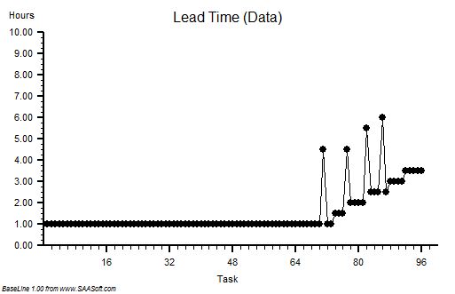
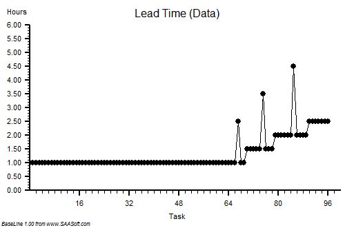
Processes imply flows. The flow into a process is called demand, while the flow out of the process is called activity. What goes in must come out, so if the demand exceeds the activity then a backlog will be growing inside the process. This growing queue creates a number of undesirable effects – first it takes up space, and second it increases the time for demand to be converted into activity. This conversion time is called the lead-time.

So, to avoid a growing queue and a growing wait, there must be sufficient flow-capacity at each and every step along the process. The obvious solution is to set the average flow-capacity equal to the average demand; and we do this because we know that more flow-capacity implies more cost – and to stay in business we must keep a lid on costs!

This sounds obvious and easy but does it actually work in practice?

The surprising answer is “No”. It doesn’t.

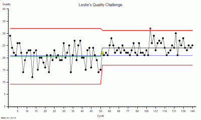
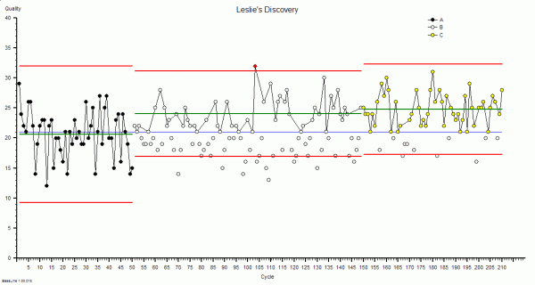
What happens in practice is that the measured average activity is always less than the funded flow-capacity, and so less than the demand. The backlogs will continue to grow; the lead-time will continue to grow; the waits will continue to grow; the internal congestion will continue to grow – until we run out of space. At that point everything can grind to a catastrophic halt. That is what we mean by a brittle process.

This fundamental and unexpected result can easily and quickly be demonstrated in a concrete way on a table top using ordinary dice and tokens. A credible game along these lines was described almost 40 years ago in The Goal by Eli Goldratt, originator of the school of improvement called Theory of Constraints. The emotional impact of gaining this insight can be profound and positive because it opens the door to a way forward which avoids the Flaw of Averages trap. There are countless success stories of using this understanding.


So, when we need to cope with variation and we choose a passive resilience approach then we have to plan to the extremes of the range of variation. Sometimes that is not possible and we are forced to accept the likelihood of failure. Or we can consider a different approach.

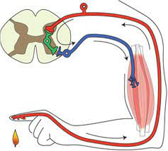
Reactive resilience is one that living systems have evolved to use extensively, and is illustrated by the simple reflex loop shown in the diagram.

A reactive system has three components linked together – a sensor (i.e. temperature sensitive nerves endings in the skin), a processor (i.e. the grey matter of the spinal chord) and an effector (i.e. the muscle, ligaments and bones). So, when a pre-defined limit of variation is reached (e.g. the flame) then the protective reaction withdraws the finger before it becomes damaged. The advantage this type of reactive resilience is that it is relatively simple and relatively fast. The disadvantage is that it is not addressing the cause of the problem.

This is called reactive, automatic and agnostic.

The automatic self-regulating systems that we see in biology, and that we have emulated in our machines, are evidence of the effectiveness of a combination of passive and reactive resilience. It is good enough for most scenarios – so long as the context remains stable. The problem comes when the context is evolving, and in that case the automatic/reflex/blind/agnostic approach will fail – at some point.


Survival in an evolving context requires more – it requires proactive resilience.

What that means is that the processor component of the feedback loop gains an extra feature – a memory. The advantage this brings is that past experience can be recalled, reflected upon and used to guide future expectation and future behaviour. We can listen and learn and become proactive. We can look ahead and we can keep up with our evolving context. One might call, this reactive adaptation or co-evolution and it is a widely observed phenomenon in nature.

The usual manifestation is this called competition.

Those who can reactively adapt faster and more effectively than others have a better chance of not failing – i.e. a better chance of survival. The traditional term for this is survival of the fittest but the trendier term for proactive resilience is agile.

And that is what successful organisations are learning to do. They are adding a layer of proactive resilience on top of their reactive resilience and their passive resilience.

All three layers of resilience are required to survive in an evolving context.

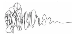
One manifestation of this is the concept of design which is where we create things with the required resilience before they are needed. This is illustrated by the design squiggle which has time running left to right and shows the design evolving adaptively until there is sufficient clarity to implement and possibly automate.

And one interesting thing about design is that it can be done without an understanding of how something works – just knowing what works is enough. The elegant and durable medieval cathedrals were designed and built by Master builders who had no formal education. They learned the heuristics as apprentices and through experience.


And if we project the word game forwards we might anticipate a form of resilience called proactive adaptation. However, we sense that is a novel thing because there is no proadaptive word in the dictionary.

PS. We might also use the term Anti-Fragile, which is the name of a thought-provoking book that explores this very topic.

The Six Dice Game

<Ring Ring><Ring Ring>

?Hello, you are through to the Improvement Science Helpline. How can we help?

This is Leslie, one of your FISH apprentices.  Could I speak to Bob – my ISP coach?

?Yes, Bob is free. I will connect you now.

<Ring Ring><Ring Ring>

?Hello Leslie, Bob here. How can I help?

Hi Bob, I have a problem that I do not feel my Foundation training has equipped me to solve. Can I talk it through with you?

?Of course. Can you outline the context for me?

Yes. The context is a department that is delivering an acceptable quality-of-service and is delivering on-time but is failing financially. As you know we are all being forced to adopt austerity measures and I am concerned that if their budget is cut then they will fail on delivery and may start cutting corners and then fail on quality too.  We need a win-win-win outcome and I do not know where to start with this one.

?OK – are you using the 6M Design method?

Yes – of course!

?OK – have you done The 4N Chart for the customer of their service?

Yes – it was their customers who asked me if I could help and that is what I used to get the context.

?OK – have you done The 4N Chart for the department?

Yes. And that is where my major concerns come from. They feel under extreme pressure; they feel they are working flat out just to maintain the current level of quality and on-time delivery; they feel undervalued and frustrated that their requests for more resources are refused; they feel demoralized; demotivated and scared that their service may be ‘outsourced’. On the positive side they feel that they work well as a team and are willing to learn. I do not know what to do next.

?OK. Do not panic. This sounds like a very common and treatable system illness.  It is a stream design problem which may be the reason your Foundation training feels insufficient. Would you like to see how a Practitioner would approach this?

Yes please!

?OK. Have you mapped their internal process?

Yes. It is a six-step process for each job. Each step has different requirements and are done by different people with different skills. In the past they had a problem with poor service quality so extra safety and quality checks were imposed by the Governance department.  Now the quality of each step is measured on a 1-6 scale and the quality of the whole process is the sum of the individual steps so is measured on a scale of 6 to 36. They now have been given a minimum quality target of 21 to achieve for every job. How they achieve that is not specified – it was left up to them.

?OK – do they record their quality measurement data?

Yes – I have their report.

?OK – how is the information presented?

As an average for the previous month which is reported up to the Quality Performance Committee.

?OK – what was the average for last month?

Their results were 24 – so they do not have an issue delivering the required quality. The problem is the costs they are incurring and they are being labelled by others as ‘inefficient’. Especially the departments who are in budget and are annoyed that this department keeps getting ‘bailed out’.

?OK. One issue here is the quality reporting process is not alerting you to the real issue. It sounds from what you say that you have fallen into the Flaw of Averages trap.

I don’t understand. What is the Flaw of Averages trap?

?The answer to your question will become clear. The finance issue is a symptom – an effect – it is unlikely to be the cause. When did this finance issue appear?

Just after the Safety and Quality Review. They needed to employ more agency staff to do the extra work created by having to meet the new Minimum Quality target.

?OK. I need to ask you a personal question. Do you believe that improving quality always costs more?

I have to say that I am coming to that conclusion. Our Governance and Finance departments are always arguing about it. Governance state ‘a minimum standard of safety and quality is not optional’ and finance say ‘but we are going out of business’. They are at loggerheads. The departments get caught in the cross-fire.

?OK. We will need to use reality to demonstrate that this belief is incorrect. Rhetoric alone does not work. If it did then we would not be having this conversation. Do you have the raw data from which the averages are calculated?

Yes. We have the data. The quality inspectors are very thorough!

?OK – can you plot the quality scores for the last fifty jobs as a BaseLine chart?

Yes – give me a second. The average is 24 as I said.

?OK – is the process stable?

Yes – there is only one flag for the fifty. I know from my FISH training that is not a cause for alarm.

?OK – what is the process capability?

I am sorry – I don’t know what you mean by that?

?My apologies. I forgot that you have not completed the Practitioner training yet. The capability is the range between the red lines on the chart.

Um – the lower line is at 17 and the upper line is at 31.

?OK – how many points lie below the target of 21.

None of course. They are meeting their Minimum Quality target. The issue is not quality – it is money.

There was a pause.  Leslie knew from experience that when Bob paused there was a surprise coming.

?Can you email me your chart?

A cold-shiver went down Leslie’s back. What was the problem here? Bob had never asked to see the data before.

Sure. I will send it now.  The recent fifty is on the right, the data on the left is from after the quality inspectors went in and before the the Minimum Quality target was imposed. This is the chart that Governance has been using as evidence to justify their existence because they are claiming the credit for improving the quality.

?OK – thanks. I have got it – let me see.  Oh dear.

Leslie was shocked. She had never heard Bob use language like ‘Oh dear’.

There was another pause.

?Leslie, what is the context for this data? What does the X-axis represent?

Leslie looked at the chart again – more closely this time. Then she saw what Bob was getting at. There were fifty points in the first group, and about the same number in the second group. That was not the interesting part. In the first group the X-axis went up to 50 in regular steps of five; in the second group it went from 50 to just over 149 and was no longer regularly spaced. Eventually she replied.

Bob, that is a really good question. My guess it is that this is the quality of the completed work.

?It is unwise to guess. It is better to go and see reality.

You are right. I knew that. It is drummed into us during the Foundation training! I will go and ask. Can I call you back?

?Of course. I will email you my direct number.


[reveal heading=”Click here to read the rest of the story“]


<Ring Ring><Ring Ring>

?Hello, Bob here.

Bob – it is Leslie. I am  so excited! I have discovered something amazing.

?Hello Leslie. That is good to hear. Can you tell me what you have discovered?

I have discovered that better quality does not always cost more.

?That is a good discovery. Can you prove it with data?

Yes I can!  I am emailing you the chart now.

?OK – I am looking at your chart. Can you explain to me what you have discovered?

Yes. When I went to see for myself I saw that when a job failed the Minimum Quality check at the end then the whole job had to be re-done because there was no time to investigate and correct the causes of the failure.  The people doing the work said that they were helpless victims of errors that were made upstream of them – and they could not predict from one job to the next what the error would be. They said it felt like quality was a lottery and that they were just firefighting all the time. They knew that just repeating the work was not solving the problem but they had no other choice because they were under enormous pressure to deliver on-time as well. The only solution they could see is was to get more resources but their requests were being refused by Finance on the grounds that there is no more money. They felt completely trapped.

?OK. Can you describe what you did?

Yes. I saw immediately that there were so many sources of errors that it would be impossible for me to tackle them all. So I used the tool that I had learned in the Foundation training: the Niggle-o-Gram. That focussed us and led to a surprisingly simple, quick, zero-cost process design change. We deliberately did not remove the Inspection-and-Correction policy because we needed to know what the impact of the change would be. Oh, and we did one other thing that challenged the current methods. We plotted both the successes and the failures on the BaseLine chart so we could see both the the quality and the work done on one chart.  And we updated the chart every day and posted it chart on the notice board so everyone in the department could see the effect of the change that they had designed. It worked like magic! They have already slashed their agency staff costs, the whole department feels calmer and they are still delivering on-time. And best of all they now feel that they have the energy and time to start looking at the next niggle. Thank you so much! Now I see how the tools and techniques I learned in FISH school are so powerful and now I understand better the reason we learned them first.

?Well done Leslie. You have taken an important step to becoming a fully fledged Improvement Science Practitioner. There are many more but you have learned some critical lessons in this challenge.


This scenario is fictional but realistic.

And it has been designed so that it can be replicated easily using a simple game that requires only pencil, paper and some dice.

If you do not have some dice handy then you can use this little program that simulates rolling six dice.

The Six Digital Dice program (for PC only).

Instructions
1. Prepare a piece of A4 squared paper with the Y-axis marked from zero to 40 and the X-axis from 1 to 80.
2. Roll six dice and record the score on each (or one die six times) – then calculate the total.
3. Plot the total on your graph. Left-to-right in time order. Link the dots with lines.
4. After 25 dots look at the chart. It should resemble the leftmost data in the charts above.
5. Now draw a horizontal line at 21. This is the Minimum Quality Target.
6. Keep rolling the dice – six per cycle, adding the totals to the right of your previous data.

But this time if the total is less than 21 then repeat the cycle of six dice rolls until the score is 21 or more. Record on your chart the output of all the cycles – not just the acceptable ones.

7. Keep going until you have 25 acceptable outcomes. As long as it takes.

Now count how many cycles you needed to complete in order to get 25 acceptable outcomes.  You should find that it is about twice as many as before you “imposed” the Inspect-and-Correct QI policy.

This illustrates the problem of an Inspection-and-Correction design for quality improvement.  It does improve the quality of the output – but at a higher cost.  We are treating the symptoms and ignoring the disease.

The internal design of the process is unchanged – and it is still generating mistakes.

How much quality improvement you get and how much it costs you is determined by the design of the underlying process – which has not changed. There is a Law of Diminishing returns here – and a risk.

The risk is that if quality improves as the result of applying a quality target then it encourages the Governance thumbscrews to be tightened further and forces the people further into cross-fire between Governance and Finance.

The other negative consequence of the Inspection-and-Correction approach is that it increases both the average and the variation in lead time which also fuels the calls for more targets, more sticks, calls for  more resources and pushes costs up even further.

The lesson from this simple reality check seems clear.

The better strategy for improving quality is to design the root causes of errors out of the processes  because then we will get improved quality and improved delivery and improved productivity and we will discover that we have improved safety as well.

The Six Dice Game is a simpler version of the famous Red Bead Game that W Edwards Deming used to explain why the arbitrary-target-driven-stick-and-carrot style of management creates more problems than it solves.

The illusion of short-term gain but the reality of long-term pain.

And if you would like to see and hear Deming talking about the science of improvement there is a video of him speaking in 1984. He is at the bottom of the page.  Click here.

[/reveal]

What Is The Cost Of Reality?

It is often assumed that “high quality costs more” and there is certainly ample evidence to support this assertion: dinner in a high quality restaurant commands a high price. The usual justifications for the assumption are (a) quality ingredients and quality skills cost more to provide; and (b) if people want a high quality product or service that is in relatively short supply then it commands a higher price – the Law of Supply and Demand.  Together this creates a self-regulating system – it costs more to produce and so long as enough customers are prepared to pay the higher price the system works.  So what is the problem? The problem is that the model is incorrect. The assumption is incorrect.  Higher quality does not always cost more – it usually costs less. Convinced?  No. Of course not. To be convinced we need hard, rational evidence that disproves our assumption. OK. Here is the evidence.

Suppose we have a simple process that has been designed to deliver the Perfect Service – 100% quality, on time, first time and every time – 100% dependable and 100% predictable. We choose a Service for our example because the product is intangible and we cannot store it in a warehouse – so it must be produced as it is consumed.

To measure the Cost of Quality we first need to work out the minimum price we would need to charge to stay in business – the sum of all our costs divided by the number we produce: our Minimum Viable Price. When we examine our Perfect Service we find that it has three parts – Part 1 is the administrative work: receiving customers; scheduling the work; arranging for the necessary resources to be available; collecting the payment; having meetings; writing reports and so on. The list of expenses seems endless. It is the necessary work of management – but it is not what adds value for the customer. Part 3 is the work that actually adds the value – it is the part the customer wants – the Service that they are prepared to pay for. So what is Part 2 work? This is where our customers wait for their value – the queue. Each of the three parts will consume resources either directly or indirectly – each has a cost – and we want Part 3 to represent most of the cost; Part 2 the least and Part 1 somewhere in between. That feels realistic and reasonable. And in our Perfect Service there is no delay between the arrival of a customer and starting the value work; so there is  no queue; so no work in progress waiting to start, so the cost of Part 2 is zero.  

The second step is to work out the cost of our Perfect Service – and we could use algebra and equations to do that but we won’t because the language of abstract mathematics excludes too many people from the conversation – let us just pick some realistic numbers to play with and see what we discover. Let us assume Part 1 requires a total of 30 mins of work that uses resources which cost £12 per hour; and let us assume Part 3 requires 30 mins of work that uses resources which cost £60 per hour; and let us assume Part 2 uses resources that cost £6 per hour (if we were to need them). We can now work out the Minimum Viable Price for our Perfect Service:

Part 1 work: 30 mins @ £12 per hour = £6
Part 2 work:  = £0
Part 3 work: 30 mins at £60 per hour = £30
Total: £36 per customer.

Our Perfect Service has been designed to deliver at the rate of demand which is one job every 30 mins and this means that the Part 1 and Part 3 resources are working continuously at 100% utilisation. There is no waste, no waiting, and no wobble. This is our Perfect Service and £36 per job is our Minimum Viable Price.         

The third step is to tarnish our Perfect Service to make it more realistic – and then to do whatever is necessary to counter the necessary imperfections so that we still produce 100% quality. To the outside world the quality of the service has not changed but it is no longer perfect – they need to wait a bit longer, and they may need to pay a bit more. Quality costs remember!  The question is – how much longer and how much more? If we can work that out and compare it with our Minimim Viable Price we will get a measure of the Cost of Reality.

We know that variation is always present in real systems – so let the first Dose of Reality be the variation in the time it takes to do the value work. What effect does this have?  This apparently simple question is surprisingly difficult to answer in our heads – and we have chosen not to use “scarymatics” so let us run an empirical experiment and see what happens. We could do that with the real system, or we could do it on a model of the system.  As our Perfect Service is so simple we can use a model. There are lots of ways to do this simulation and the technique used in this example is called discrete event simulation (DES)  and I used a process simulation tool called CPS (www.SAASoft.com).

Let us see what happens when we add some random variation to the time it takes to do the Part 3 value work – the flow will not change, the average time will not change, we will just add some random noise – but not too much – something realistic like 10% say.

The chart shows the time from start to finish for each customer and to see the impact of adding the variation the first 48 customers are served by our Perfect Service and then we switch to the Realistic Service. See what happens – the time in the process increases then sort of stabilises. This means we must have created a queue (i.e. Part 2 work) and that will require space to store and capacity to clear. When we get the costs in we work out our new minimum viable price it comes out, in this case, to be £43.42 per task. That is an increase of over 20% and it gives us a measure of the Cost of the Variation. If we repeat the exercise many times we get a similar answer, not the same every time because the variation is random, but it is always an extra cost. It is never less that the perfect proce and it does not average out to zero. This may sound counter-intuitive until we understand the reason: when we add variation we need a bit of a queue to ensure there is always work for Part 3 to do; and that queue will form spontaneously when customers take longer than average. If there is no queue and a customer requires less than average time then the Part 3 resource will be idle for some of the time. That idle time cannot be stored and used later: time is not money.  So what happens is that a queue forms spontaneously, so long as there is space for it,  and it ensures there is always just enough work waiting to be done. It is a self-regulating system – the queue is called a buffer.

Let us see what happens when we take our Perfect Process and add a different form of variation – random errors. To prevent the error leaving the system and affecting our output quality we will repeat the work. If the errors are random and rare then the chance of getting it wrong twice for the same customer will be small so the rework will be a rough measure of the internal process quality. For a fair comparison let us use the same degree of variation as before – 10% of the Part 3 have an error and need to be reworked – which in our example means work going to the back of the queue.

Again, to see the effect of the change, the first 48 tasks are from the Perfect System and after that we introduce a 10% chance of a task failing the quality standard and needing to be reworked: in this example 5 tasks failed, which is the expected rate. The effect on the start to finish time is very different from before – the time for the reworked tasks are clearly longer as we would expect, but the time for the other tasks gets longer too. It implies that a Part 2 queue is building up and after each error we can see that the queue grows – and after a delay.  This is counter-intuitive. Why is this happening? It is because in our Perfect Service we had 100% utiliation – there was just enough capacity to do the work when it was done right-first-time, so if we make errors and we create extra demand and extra load, it will exceed our capacity; we have created a bottleneck and the queue will form and it will cointinue to grow as long as errors are made.  This queue needs space to store and capacity to clear. How much though? Well, in this example, when we add up all these extra costs we get a new minimum price of £62.81 – that is a massive 74% increase!  Wow! It looks like errors create much bigger problem for us than variation. There is another important learning point – random cycle-time variation is self-regulating and inherently stable; random errors are not self-regulating and they create inherently unstable processes.

Our empirical experiment has demonstrated three principles of process design for minimising the Cost of Reality:

1. Eliminate sources of errors by designing error-proofed right-first-time processes that prevent errors happening.
2. Ensure there is enough spare capacity at every stage to allow recovery from the inevitable random errors.
3. Ensure that all the steps can flow uninterrupted by allowing enough buffer space for the critical steps.

With these Three Principles of cost-effective design in mind we can now predict what will happen if we combine a not-for-profit process, with a rising demand, with a rising expectation, with a falling budget, and with an inspect-and-rework process design: we predict everyone will be unhappy. We will all be miserable because the only way to stay in budget is to cut the lower priority value work and reinvest the savings in the rising cost of checking and rework for the higher priority jobs. But we have a  problem – our activity will fall, so our revenue will fall, and despite the cost cutting the budget still doesn’t balance because of the increasing cost of inspection and rework – and we enter the death spiral of finanical decline.

The only way to avoid this fatal financial tailspin is to replace the inspection-and-rework habit with a right-first-time design; before it is too late. And to do that we need to learn how to design and deliver right-first-time processes.

Charts created using BaseLine

The Crime of Metric Abuse

We live in a world that is increasingly intolerant of errors – we want everything to be right all the time – and if it is not then someone must have erred with deliberate intent so they need to be named, blamed and shamed! We set safety standards and tough targets; we measure and check; and we expose and correct anyone who is non-conformant. We accept that is the price we must pay for a Perfect World … Yes? Unfortunately the answer is No. We are deluded. We are all habitual criminals. We are all guilty of committing a crime against humanity – the Crime of Metric Abuse. And we are blissfully ignorant of it so it comes as a big shock when we learn the reality of our unconscious complicity.

You might want to sit down for the next bit.

First we need to set the scene:
1. Sustained improvement requires actions that result in irreversible and beneficial changes to the structure and function of the system.
2. These actions require making wise decisions – effective decisions.
3. These actions require using resources well – efficient processes.
4. Making wise decisions requires that we use our system metrics correctly.
5. Understanding what correct use is means recognising incorrect use – abuse awareness.

When we commit the Crime of Metric Abuse, even unconsciously, we make poor decisions. If we act on those decisions we get an outcome that we do not intend and do not want – we make an error.  Unfortunately, more efficiency does not compensate for less effectiveness – if fact it makes it worse. Efficiency amplifies Effectiveness – “Doing the wrong thing right makes it wronger not righter” as Russell Ackoff succinctly puts it.  Paradoxically our inefficient and bureaucratic systems may be our only defence against our ineffective and potentially dangerous decision making – so before we strip out the bureaucracy and strive for efficiency we had better be sure we are making effective decisions and that means exposing and treating our nasty habit for Metric Abuse.

Metric Abuse manifests in many forms – and there are two that when combined create a particularly virulent addiction – Abuse of Ratios and Abuse of Targets. First let us talk about the Abuse of Ratios.

A ratio is one number divided by another – which sounds innocent enough – and ratios are very useful so what is the danger? The danger is that by combining two numbers to create one we throw away some information. This is not a good idea when making the best possible decision means squeezing every last drop of understanding our of our information. To unconsciously throw away useful information amounts to incompetence; to consciously throw away useful information is negligence because we could and should know better.

Here is a time-series chart of a process metric presented as a ratio. This is productivity – the ratio of an output to an input – and it shows that our productivity is stable over time.  We started OK and we finished OK and we congratulate ourselves for our good management – yes? Well, maybe and maybe not.  Suppose we are measuring the Quality of the output and the Cost of the input; then calculating our Value-For-Money productivity from the ratio; and then only share this derived metric. What if quality and cost are changing over time in the same direction and by the same rate? The productivity ratio will not change.


Suppose the raw data we used to calculate our ratio was as shown in the two charts of measured Ouput Quality and measured Input Cost  – we can see immediately that, although our ratio is telling us everything is stable, our system is actually changing over time – it is unstable and therefore it is unpredictable. Systems that are unstable have a nasty habit of finding barriers to further change and when they do they have a habit of crashing, suddenly, unpredictably and spectacularly. If you take your eyes of the white line when driving and drift off course you may suddenly discover a barrier – the crash barrier for example, or worse still an on-coming vehicle! The apparent stability indicated by a ratio is an illusion or rather a delusion. We delude ourselves that we are OK – in reality we may be on a collision course with catastrophe. 

But increasing quality is what we want surely? Yes – it is what we want – but at what cost? If we use the strategy of quality-by-inspection and add extra checking to detect errors and extra capacity to fix the errors we find then we will incur higher costs. This is the story that these Quality and Cost charts are showing.  To stay in business the extra cost must be passed on to our customers in the price we charge: and we have all been brainwashed from birth to expect to pay more for better quality. But what happens when the rising price hits our customers finanical constraint?  We are no longer able to afford the better quality so we settle for the lower quality but affordable alternative.  What happens then to the company that has invested in quality by inspection? It loses customers which means it loses revenue which is bad for its financial health – and to survive it starts cutting prices, cutting corners, cutting costs, cutting staff and eventually – cutting its own throat! The delusional productivity ratio has hidden the real problem until a sudden and unpredictable drop in revenue and profit provides a reality check – by which time it is too late. Of course if all our competitors are committing the same crime of metric abuse and suffering from the same delusion we may survive a bit longer in the toxic mediocrity swamp – but if a new competitor who is not deluded by ratios and who learns how to provide consistently higher quality at a consistently lower price – then we are in big trouble: our customers leave and our end is swift and without mercy. Competition cannot bring controlled improvement while the Abuse of Ratios remains rife and unchallenged.

Now let us talk about the second Metric Abuse, the Abuse of Targets.

The blue line on the Productivity chart is the Target Productivity. As leaders and managers we have bee brainwashed with the mantra that “you get what you measure” and with this belief we commit the crime of Target Abuse when we set an arbitrary target and use it to decide when to reward and when to punish. We compound our second crime when we connect our arbitrary target to our accounting clock and post periodic praise when we are above target and periodic pain when we are below. We magnify the crime if we have a quality-by-inspection strategy because we create an internal quality-cost tradeoff that generates conflict between our governance goal and our finance goal: the result is a festering and acrimonious stalemate. Our quality-by-inspection strategy paradoxically prevents improvement in productivity and we learn to accept the inevitable oscillation between good and bad and eventually may even convince ourselves that this is the best and the only way.  With this life-limiting-belief deeply embedded in our collective unconsciousness, the more enthusiastically this quality-by-inspection design is enforced the more fear, frustration and failures it generates – until trust is eroded to the point that when the system hits a problem – morale collapses, errors increase, checks are overwhelmed, rework capacity is swamped, quality slumps and costs escalate. Productivity nose-dives and both customers and staff jump into the lifeboats to avoid going down with the ship!  

The use of delusional ratios and arbitrary targets (DRATs) is a dangerous and addictive behaviour and should be made a criminal offense punishable by Law because it is both destructive and unnecessary.

With painful awareness of the problem a path to a solution starts to form:

1. Share the numerator, the denominator and the ratio data as time series charts.
2. Only put requirement specifications on the numerator and denominator charts.
3. Outlaw quality-by-inspection and replace with quality-by-design-and-improvement.  

Metric Abuse is a Crime. DRATs are a dangerous addiction. DRATs kill Motivation. DRATs Kill Organisations.

Charts created using BaseLine

JIT, WIP, LIP and PIP

It is a fantastic feeling when a piece of the jigsaw falls into place and suddenly an important part of the bigger picture emerges. Feelings of confusion, anxiety and threat dissipate and are replaced by a sense of insight, calm and opportunitity.

Improvement Science is about 80% subjective and 20% objective: more cultural than technical – but the technical parts are necessary. Processes obey the Laws of Physics – and unlike the Laws of People these not open to appeal or repeal. So when an essential piece of process physics is missing the picture is incomplete and confusion reigns.

One piece of the process physics jigsaw is JIT (Just-In-Time) and process improvement zealots rant on about JIT as if it were some sort of Holy Grail of Improvement Science.  JIT means what you need arrives just when you need it – which implies that there is no waiting of it-for-you or you-for-it.  JIT is an important output of an improved process; it is not an input!  The danger of confusing output with input is that we may then try to use delivery time as a mangement metric rather than a performance metric – and if we do that we get ourselves into a lot of trouble. Delivery time targets are often set and enforced and to a large extent fail to achieve their intention because of this confusion.  To understand how to achieve JIT requires more pieces of the process physics jigsaw. The piece that goes next to JIT is labelled WIP (Work In Progress) which is the number of jobs that are somewhere between starting and finishing.  JIT is achieved when WIP is low enough to provide the process with just the right amount of resilience to absorb inevitable variation; and WIP is a more useful management metric than JIT for many reasons (which for brevity I will not explain here). Monitoring WIP enables a process manager to become more proactive because changes in WIP can signal a future problem with JIT – giving enough warning to do something.  However, although JIT and WIP are necessary they are not sufficient – we need a third piece of the jigsaw to allow us to design our process to deliver the JIT performance we want.  This third piece is called LIP (Load-In-Progress) and is the parameter needed to plan and schedule  the right capacity at the right place and the right time to achieve the required WIP and JIT.  Together these three pieces provide the stepping stones on the path to Productivity Improvement Planning (PIP) that is the combination of QI (Quality Improvement) and CI (Cost Improvement).

So if we want our PIP then we need to know our LIP and WIP to get the JIT.  Reddit? Geddit?         

Is a Queue an Asset or a Liability?

Many believe that a queue is a good thing.

To a supplier a queue is tangible evidence that there is demand for their product or service and reassurance that their resources will not sit idle, waiting for work and consuming profit rather than creating it.  To a customer a queue is tangible evidence that the product or service is in demand and therefore must be worth having. They may have to wait but the wait will be worth it.  Both suppliers and customers unconsciously collude in the Great Deception and even give it a name – “The Law of Supply and Demand”. By doing so they unwittingly open the door for charlatans and tricksters who deliberately create and maintain queues to make themselves appear more worthy or efficient than they really are.

Even though we all know this intuitively we seem unable to do anything about it. “That is just the way it is” we say with a shrug of resignation. But it does not have to be so – there is a path out of this dead end.

Let us look at this problem from a different perspective. Is a product actually any better because we have waited to get it? No. A longer wait does not increase the quality of the product or service and may indeed impair it.  So, if  a queue does not increase quality does it reduce the cost?  The answer again is “No”. A queue always increases the cost and often in many ways.  Exactly how much the cost increases by depends on what is on the queue, where the queue is, and how long it is. This may sound counter-intitutive and didactic so I need to explain in a bit more detail the reason this statement is an inevitable consequence of the Laws of Physics.

Suppose the queue comprises perishable goods; goods that require constant maintenance; goods that command a fixed price when they leave the queue; goods that are required to be held in a container of limited capacity with fixed overhead costs (i.e. costs that are fixed irrespective of how full the container is).  Patients in a hospital or passengers on an aeroplane are typical examples because the patient/passenger is deprived of their ability to look after themselves; they are totally dependent on others for supplying all their basic needs; and they are perishable in the sense that a patient cannot wait forever for treatment and an aeroplane cannot fly around forever waiting to land. A queue of patients waiting to leave hospital or an aeroplane full of passsengers circling to land at an airport represents an expensive queue – the queue has a cost – and the bigger the queue is and the longer it persists the greater the cost.

So how does a queue form in the first place? The answer is: when the flow in exceeds the flow out. The instant that happens the queue starts to grow bigger.  When flow in is less than flow out the queue is getting smaller – but we cannot have a negative queue – so when the flow out exceeds the flow in AND the size of the queue reaches zero the system suddenly changes behaviour – the work dries up and the resources become idle.  This creates a different cost – the cost of idle resources consuming money but not producing revenue. So a queue/work costs and no queue/no work costs too.  The least cost situation is when the work arrives at exactly the same rate that it can be done: there is no waiting by anyone – no queue and no idle resources.  Note however that this does not imply that the work has to arrive at a constant rate – only that rate at which the work arrives matches the rate at which it is done – it is the difference between the two that should be zero at all times. And where we have several steps – the flow must be the same through all steps of the stream at all times.  Remember the second condition for minimum cost – the size of the queue must be zero as well – this is the zero inventory goal of the “perfect process”.

So, if any deviation from this perfect balance of flow creates some form of cost, why do we ever tolerate queues? The reason is that the perfect world above implies that it is possible to predict the flow in and the flow out with complete accuracy and reliabilty.  We all know from experience that this is impossible: there is always some degree of  natural variation which is unpredictable and which we often call “noise” or “chaos”. For that single reason the lowest cost (not zero cost) situation is when there is just enough breathing space for a queue to wax and wane – smoothing out the unpredictable variation between inflow and outflow. This healthy queue is called a buffer.

The less “noise” the less breathing space is needed and the closer you can get to zero queue cost.

So, given this logical explanation it might surprise you to learn that most of the flow variation we observe in real processes is neither natural nor unpredictable – we deliberately and persistently inject predictable flow variation into our processes.  This unnatural variation is created by own policies – for example, accumulating DIY jobs until there are enough to justify doing them.   The reason we do this is because we have been bamboozled into believing it is a good thing for the financial health of our system. We have been beguiled by the accountants – the Money Magicians.  Actually that is not precise enough – the accountants themselves  are the innocent messengers – the deception comes from the Accounting Policies.  The major niggle is one convention that has become ossified into Accounting Practice – the convention that a queue of work waiting to be finished or sold represents an asset – sort of frozen-for-now-cash that can be thawed out or “liquidated” when the product is sold.  This convention is not incorrect it is just incomplete because, as we have demonstrated, every queue incurs a cost.  In accountant-speak a cost is called a liability and unfortunately this queue-cost-liability is never included in the accounts and this makes a very, very, big difference to the outcome. To assess the financial health of an organisation at a point in time an accountant will use a balance sheet to subtract the liabilities from the assets and come up with a number that is called equity. If that number is zero or negative then the business is financially dead – the technical name is bankruptcy and no accountant likes to utter the B word.  Denial is not a reliable long term buisness strategy and if our Accounting Policies do not include the cost of the queue as a liability on the balance sheet then our finanical reports will be a distortion of reality and will present the business as healthier than it really is.  This is an Error of Omission and has grave negative consequences.  One of which is that it can create a sense of complacency, a blindness to the early warning signs of financial illness and reactive rather than proactive behaviour. The problem is compounded when a large and complex organisation is split into smaller, simpler mini-businesses that all suffer from the same financial blindspot. It becomes even more difficult to see the problem when everyone is making the same error of omission and when it is easier to blame someone else for the inevitable problems that ensue.

We all know from experience that prevention is better than cure and we also know that the future is not predictable with certainty: so in addition to prevention we need vigilence, prompt action, decisive action and appropriate action at the earliest detectable sign of a significant deterioration. Complacency is not a reliable long term survival strategy.

So what is the way forward? Dispense with the accountants? NO! You need them – they are very good at what they do – it is just that what they are doing is not exactly what we all need them to be doing – and that is because the Accounting Policies that they diligently enforce are incomplete.  A safer strategy would be for us to set our accountants the task of learning how to count the cost of a queue and to include that in our internal finanical reporting. The quality of business decisions based on financial data will improve and that is good for everyone – the business, the customers and the reputation of the Accounting Profession. Win-win-win.

The question was “Is a queue and asset or a liability?” The answer is “Both”.

How Do We Measure the Cost of Waste?

There is a saying in Yorkshire “Where there’s muck there’s brass” which means that muck or waste is expensive to create and to clean up. 

Improvement science provides the theory, techniques and tools to reduce the cost of waste and to re-invest the savings in further improvement.  But how much does waste cost us? How much can we expect to release to re-invest?  The answer is deceptively simple to work out and decidedly alarming when we do.

We start with the conventional measurement of cost – the expenses – be they materials, direct labour, indirect labour, whatever. We just add up all the costs for a period of time to give the total spend – let us call that the stage cost. The next step requires some new thinking – it requires looking from the perspective of the job or customer – and following the path backwards from the intended outcome, recording what was done, how much resource-time and material it required and how much that required work actually cost.  This is what one satisfied customer is prepared to pay for; so let us call this the required stream cost. We now just multiply the output or activity for the period of time by the required stream cost and we will call that the total stream cost. We now just compare the stage cost and the stream cost – the difference is the cost of waste – the cost of all the resources consumed that did not contribute to the intended outcome. The difference is usually large; the stream cost is typically only 20%-50% of the stage cost!

This may sound unbelieveable but it is true – and the only way to prove it to go and observe the process and do the calculation – just looking at our conventional finanical reports will not give us the answer.  Once we do this simple experiment we will see the opportunity that Improvement Science offers – to reduce the cost of waste in a planned and predictable manner.

But if we are not prepared to challenge our assumptions by testing them against reality then we will deny ourselves that opportunity. The choice is ours.

One of the commonest assumptions we make is called the Flaw of Averages: the assumption that it is always valid to use averages when developing business cases. This assumption is incorrect.  But it is not immediately obvious why it is incorrect and the explanation sounds counter-intuitive. So, one way to illustrate is with a real example and here is one that has been created using a process simulation tool – virtual reality: