BaseLine – HCSE Blog

20/10/201206/01/2024

Look Out For The Time Trap!

There is a common system ailment which every Improvement Scientist needs to know how to manage.

In fact, it is probably the commonest.

The Symptoms: Disappointingly long waiting times and all resources running flat out.

The Diagnosis? 90%+ of managers say “It is obvious – lack of capacity!”.

The Treatment? 90%+ of managers say “It is obvious – more capacity!!”

Intuitively obvious maybe – but unfortunately these are incorrect answers. Which implies that 90%+ of managers do not understand how their systems work. That is a bit of a worry. Lament not though – misunderstanding is a treatable symptom of an endemic system disease called agnosia (=not knowing).

The correct answer is “I do not yet have enough information to make a diagnosis“.

This answer is more helpful than it looks because it prompts four other questions:

Q1. “What other possible system diagnoses are there that could cause this pattern of symptoms?”
Q2. “What do I need to know to distinguish these system diagnoses?”
Q3. “How would I treat the different ones?”
Q4. “What is the risk of making the wrong system diagnosis and applying the wrong treatment?”

Before we start on this list we need to set out a few ground rules that will protect us from more intuitive errors (see last week).

The first Rule is this:

Rule #1: Data without context is meaningless.

For example 130 is a number – it is data. 130 what? 130 mmHg. Ah ha! The “mmHg” is the units – it means millimetres of mercury and it tells us this data is a pressure. But what, where, when,who, how and why? We need more context.

“The systolic blood pressure measured in the left arm of Joe Bloggs, a 52 year old male, using an Omron M2 oscillometric manometer on Saturday 20th October 2012 at 09:00 is 130 mmHg”.

The extra context makes the data much more informative. The data has become information.

To understand what the information actually means requires some prior knowledge. We need to know what “systolic” means and what an “oscillometric manometer” is and the relevance of the “52 year old male”. This ability to extract meaning from information has two parts – the ability to recognise the language – the syntax; and the ability to understand the concepts that the words are just labels for; the semantics.

To use this deeper understanding to make a wise decision to do something (or not) requires something else. Exploring that would distract us from our current purpose. The point is made.

Rule #1: Data without context is meaningless.

In fact it is worse than meaningless – it is dangerous. And it is dangerous because when the context is missing we rarely stop and ask for it – we rush ahead and fill the context gaps with assumptions. We fill the context gaps with beliefs, prejudices, gossip, intuitive leaps, and sometimes even plain guesses.

This is dangerous – because the same data in a different context may have a completely different meaning.

To illustrate. If we change one word in the context – if we change “systolic” to “diastolic” then the whole meaning changes from one of likely normality that probably needs no action; to one of serious abnormality that definitely does. If we missed that critical word out then we are in danger of assuming that the data is systolic blood pressure – because that is the most likely given the number. And we run the risk of missing a common, potentially fatal and completely treatable disease called Stage 2 hypertension.

There is a second rule that we must always apply when using data from systems. It is this:

Rule #2: Plot time-series data as a chart – a system behaviour chart (SBC).

The reason for the second rule is because the first question we always ask about any system must be “Is our system stable?”

Q: What do we mean by the word “stable”? What is the concept that this word is a label for?

A: Stable means predictable-within-limits.

Q: What limits?

A: The limits of natural variation over time.

Q: What does that mean?

A: Let me show you.

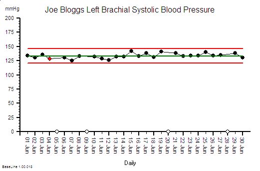
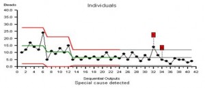
Joe Bloggs is disciplined. He measures his blood pressure almost every day and he plots the data on a chart together with some context . The chart shows that his systolic blood pressure is stable. That does not mean that it is constant – it does vary from day to day. But over time a pattern emerges from which Joe Bloggs can see that, based on past behaviour, there is a range within which future behaviour is predicted to fall. And Joe Bloggs has drawn these limits on his chart as two red lines and he has called them expectation lines. These are the limits of natural variation over time of his systolic blood pressure.

If one day he measured his blood pressure and it fell outside that expectation range then he would say “I didn’t expect that!” and he could investigate further. Perhaps he made an error in the measurement? Perhaps something else has changed that could explain the unexpected result. Perhaps it is higher than expected because he is under a lot of emotional stress a work? Perhaps it is lower than expected because he is relaxing on holiday?

His chart does not tell him the cause – it just flags when to ask more “What might have caused that?” questions.

If you arrive at a hospital in an ambulance as an emergency then the first two questions the emergency care team will need to know the answer to are “How sick are you?” and “How stable are you?”. If you are sick and getting sicker then the first task is to stabilise you, and that process is called resuscitation. There is no time to waste.

So how is all this relevant to the common pattern of symptoms from our sick system: disappointingly long waiting times and resources running flat out?

Using Rule#1 and Rule#2: To start to establish the diagnosis we need to add the context to the data and then plot our waiting time information as a time series chart and ask the “Is our system stable?” question.

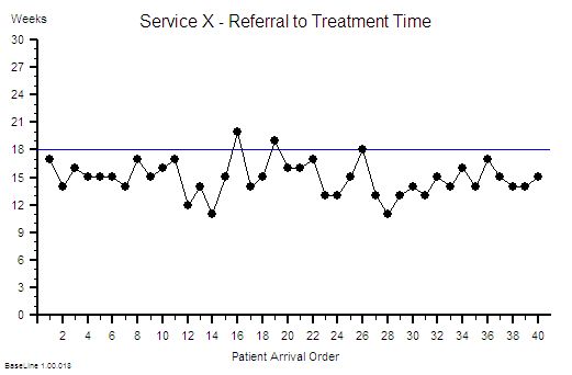
Suppose we do that and this is what we see. The context is that we are measuring the Referral-to-Treatment Time (RTT) for consecutive patients referred to a single service called X. We only know the actual RTT when the treatment happens and we want to be able to set the expectation for new patients when they are referred – because we know that if patients know what to expect then they are less likely to be disappointed – so we plot our retrospective RTT information in the order of referral. With the Mark I Eyeball Test (i.e. look at the chart) we form the subjective impression that our system is stable. It is delivering a predictable-within-limits RTT with an average of about 15 weeks and an expected range of about 10 to 20 weeks.

So far so good.

Unfortunately, the purchaser of our service has set a maximum limit for RTT of 18 weeks – a key performance indicator (KPI) target – and they have decided to “motivate” us by withholding payment for every patient that we do not deliver on time. We can now see from our chart that failures to meet the RTT target are expected, so to avoid the inevitable loss of income we have to come up with an improvement plan. Our jobs will depend on it!

Now we have a problem – because when we look at the resources that are delivering the service they are running flat out – 100% utilisation. They have no spare flow-capacity to do the extra work needed to reduce the waiting list. Efficiency drives and exhortation have got us this far but cannot take us any further. We conclude that our only option is “more capacity”. But we cannot afford it because we are operating very close to the edge. We are a not-for-profit organisation. The budgets are tight as a tick. Every penny is being spent. So spending more here will mean spending less somewhere else. And that will cause a big argument.

So the only obvious option left to us is to change the system – and the easiest thing to do is to monitor the waiting time closely on a patient-by-patient basis and if any patient starts to get close to the RTT Target then we bump them up the list so that they get priority. Obvious!

WARNING: We are now treating the symptoms before we have diagnosed the underlying disease!

In medicine that is a dangerous strategy. Symptoms are often not-specific. Different diseases can cause the same symptoms. An early morning headache can be caused by a hangover after a long night on the town – it can also (much less commonly) be caused by a brain tumour. The risks are different and the treatment is different. Get that diagnosis wrong and disappointment will follow. Do I need a hole in the head or will a paracetamol be enough?

Back to our list of questions.

What else can cause the same pattern of symptoms of a stable and disappointingly long waiting time and resources running at 100% utilisation?

There are several other process diseases that cause this symptom pattern and none of them are caused by lack of capacity.

Which is annoying because it challenges our assumption that this pattern is always caused by lack of capacity. Yes – that can sometimes be the cause – but not always.

But before we explore what these other system diseases are we need to understand why our current belief is so entrenched.

One reason is because we have learned, from experience, that if we throw flow-capacity at the problem then the waiting time will come down. When we do “waiting list initiatives” for example. So if adding flow-capacity reduces the waiting time then the cause must be lack of capacity? Intuitively obvious.

Intuitively obvious it may be – but incorrect too. We have been tricked again. This is flawed causal logic. It is called the illusion of causality.

To illustrate. If a patient complains of a headache and we give them paracetamol then the headache will usually get better. That does not mean that the cause of headaches is a paracetamol deficiency. The headache could be caused by lots of things and the response to treatment does not reliably tell us which possible cause is the actual cause. And by suppressing the symptoms we run the risk of missing the actual diagnosis while at the same time deluding ourselves that we are doing a good job.

If a system complains of long waiting times and we add flow-capacity then the long waiting time will usually get better. That does not mean that the cause of long waiting time is lack of flow-capacity. The long waiting time could be caused by lots of things. The response to treatment does not reliably tell us which possible cause is the actual cause – so by suppressing the symptoms we run the risk of missing the diagnosis while at the same time deluding ourselves that we are doing a good job.

The similarity is not a co-incidence. All systems behave in similar ways. Similar counter-intuitive ways.

So what other system diseases can cause a stable and disappointingly long waiting time and high resource utilisation?

The commonest system disease that is associated with these symptoms is a time trap – and they have nothing to do with capacity or flow.

They are part of the operational policy design of the system. And we actually design time traps into our systems deliberately! Oops!

We create a time trap when we deliberately delay doing something that we could do immediately – perhaps to give the impression that we are very busy or even overworked! We create a time trap whenever we deferring until later something we could do today.

If the task does not seem important or urgent for us then it is a candidate for delaying with a time trap.

Unfortunately it may be very important and urgent for someone else – and a delay could be expensive for them.

Creating time traps gives us a sense of power – and it is for that reason they are much loved by bureaucrats.

To illustrate how time traps cause these symptoms consider the following scenario:

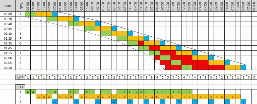
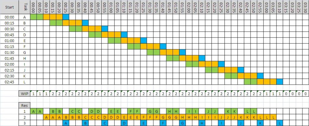
Suppose I have just enough resource-capacity to keep up with demand and flow is smooth and fault-free. My resources are 100% utilised; the flow-in equals the flow-out; and my waiting time is stable. If I then add a time trap to my design then the waiting time will increase but over the long term nothing else will change: the flow-in, the flow-out, the resource-capacity, the cost and the utilisation of the resources will all remain stable. I have increased waiting time without adding or removing capacity. So lack of resource-capacity is not always the cause of a longer waiting time.

This new insight creates a new problem; a BIG problem.

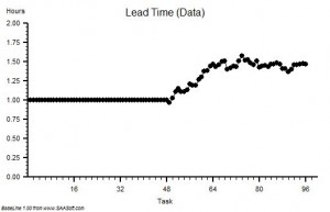
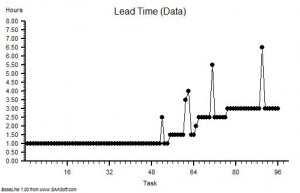
Suppose we are measuring flow-in (demand) and flow-out (activity) and time from-start-to-finish (lead time) and the resource usage (utilisation) and we are obeying Rule#1 and Rule#2 and plotting our data with its context as system behaviour charts. If we have a time trap in our system then none of these charts will tell us that a time-trap is the cause of a longer-than-necessary lead time.

Aw Shucks!

And that is the primary reason why most systems are infested with time traps. The commonly reported performance metrics we use do not tell us that they are there. We cannot improve what we cannot see.

Well actually the system behaviour charts do hold the clues we need – but we need to understand how systems work in order to know how to use the charts to make the time trap diagnosis.

Q: Why bother though?

A: Simple. It costs nothing to remove a time trap. We just design it out of the process. Our flow-in will stay the same; our flow-out will stay the same; the capacity we need will stay the same; the cost will stay the same; the revenue will stay the same but the lead-time will fall.

Q: So how does that help me reduce my costs? That is what I’m being nailed to the floor with as well!

A: If a second process requires the output of the process that has a hidden time trap then the cost of the queue in the second process is the indirect cost of the time trap. This is why time traps are such a fertile cause of excess cost – because they are hidden and because their impact is felt in a different part of the system – and usually in a different budget.

To illustrate. Suppose that 60 patients per day are discharged from our hospital and each one requires a prescription of to-take-out (TTO) medications to be completed before they can leave. Suppose that there is a time trap in this drug dispensing and delivery process. The time trap is a policy where a porter is scheduled to collect and distribute all the prescriptions at 5 pm. The porter is busy for the whole day and this policy ensures that all the prescriptions for the day are ready before the porter arrives at 5 pm. Suppose we get the event data from our electronic prescribing system (EPS) and we plot it as a system behaviour chart and it shows most of the sixty prescriptions are generated over a four hour period between 11 am and 3 pm. These prescriptions are delivered on paper (by our busy porter) and the pharmacy guarantees to complete each one within two hours of receipt although most take less than 30 minutes to complete. What is the cost of this one-delivery-per-day-porter-policy time trap? Suppose our hospital has 500 beds and the total annual expense is £182 million – that is £0.5 million per day. So sixty patients are waiting for between 2 and 5 hours longer than necessary, because of the porter-policy-time-trap, and this adds up to about 5 bed-days per day – that is the cost of 5 beds – 1% of the total cost – about £1.8 million. So the time trap is, indirectly, costing us the equivalent of £1.8 million per annum. It would be much more cost-effective for the system to have a dedicated porter working from 12 am to 5 pm doing nothing else but delivering dispensed TTOs as soon as they are ready! And assuming that there are no other time traps in the decision-to-discharge process; such as the time trap created by batching all the TTO prescriptions to the end of the morning ward round; and the time trap created by the batch of delivered TTOs waiting for the nurses to distribute them to the queue of waiting patients!

Q: So how do we nail the diagnosis of a time trap and how do we differentiate it from a Batch or a Bottleneck or Carveout?

A: To learn how to do that will require a bit more explanation of the physics of processes.

And anyway if I just told you the answer you would know how but might not understand why it is the answer. Knowledge and understanding are not the same thing. Wise decisions do not follow from just knowledge – they require understanding. Especially when trying to make wise decisions in unfamiliar scenarios.

It is said that if we are shown we will understand 10%; if we can do we will understand 50%; and if we are able to teach then we will understand 90%.

So instead of showing how instead I will offer a hint. The first step of the path to knowing how and understanding why is in the following essay:

A Study of the Relative Value of Different Time-series Charts for Proactive Process Monitoring. JOIS 2012;3:1-18

Click here to visit JOIS

24/11/2011

Pushmepullyu

The pushmepullyu is a fictional animal immortalised in the 1960’s film Dr Dolittle featuring Rex Harrison who learned from a parrot how to talk to animals. The pushmepullyu was a rare, mysterious animal that was never captured and displayed in zoos. It had a sharp-horned head at both ends and while one head slept the other stayed awake so it was impossible to sneak up on and capture.

The spirit of the pushmepullyu lives on in Improvement Science as Push-Pull and remains equally mysterious and difficult to understand and explain. It is confusing terminology. So what does Push-Pull acually mean?

To decode the terminology we need to first understand a critical metric of any process – the constraint cycle time (CCT) – and to do that we need to define what the terms constraint and cycle time mean.

Consider a process that comprises a series of steps that must be completed in sequence. If we put one task through the process we can measure how long each step takes to complete its contribution to the whole task. This is the touch time of the step and if the resource is immediately available to start the next task this is also the cycle time of the step.

If we now start two tasks at the same time then we will observe when an upstream step has a longer cycle time than the next step downstream because it will shadow the downstream step. In contrast, if the upstream step has a shorter cycle time than the next step down stream then it will expose the downstream step. The differences in the cycle times of the steps will determine the behaviour of the process.

Confused? Probably. The description above is correct BUT hard to understand because we learn better from reality than from rhetoric; and we find pictures work better than words. Pragmatic comes before academic; reality before theory. We need a realistic example to learn from.

Suppose we have a process that we are told has three steps in sequence, and when one task is put through it takes 30 mins to complete. This is called the lead time and is an important process output metric. We now know it is possible to complete the work in 30 mins so we can set this as our lead time expectation.

Suppose we plot a chart of lead times in the order that the tasks start and record the start time and lead time for each one – and we get a chart that looks like this. It is called a lead time run chart. The first six tasks complete in 30 mins as expected – then it all goes pear-shaped. But why? The run chart does not tell us the reason – it just alerts us to dig deeper.

The clue is in the run chart but we need to know what to look for. We do not know how to do that yet so we need to ask for some more data.

We are given this run chart – which is a count of the number of tasks being worked on recorded at 5 minute intervals. It is the work in progress run chart.

We know that we have a three step process and three separate resources – one for each step. So we know that that if there is a WIP of less than 3 we must have idle resources; and if there is a WIP of more than 3 we must have queues of tasks waiting.

We can see that the WIP run chart looks a bit like the lead time run chart. But it still does not tell us what is causing the unstable behaviour.

In fact we do already have all the data we need to work it out but it is not intuitively obvious how to do it. We feel we need to dig deeper.

We decide to go and see for ourselves and to observe exactly what happens to each of the twelve tasks and each of the three resources. We use these observations to draw a Gantt chart.

Now we can see what is happening.

We can see that the cycle time of Step 1 (green) is 10 mins; the cycle time for Step 2 (amber) is 15 mins; and the cycle time for Step 3 (blue) is 5 mins.

This explains why the minimum lead time was 30 mins: 10+15+5 = 30 mins. OK – that makes sense now.

Red means tasks waiting and we can see that a lead time longer than 30 mins is associated with waiting – which means one or more queues. We can see that there are two queues – the first between Step 1 and Step 2 which starts to form at Task G and then grows; and the second before Step 1 which first appears for Task J and then grows. So what changes at Task G and Task J?

Looking at the chart we can see that the slope of the left hand edge is changing – it is getting steeper – which means tasks are arriving faster and faster. We look at the interval between the start times and it confirms our suspicion. This data was the clue in the original lead time run chart.

Looking more closely at the differences between the start times we can see that the first three arrive at one every 20 mins; the next three at one every 15 mins; the next three at one every 10 mins and the last three at one every 5 mins.

Ah ha!

Tasks are being pushed into the process at an increasing rate that is independent of the rate at which the process can work.

When we compare the rate of arrival with the cycle time of each step in a process we find that one step will be most exposed – it is called the constraint step and it is the step that controls the flow in the whole process. The constraint cycle time is therefore the critical metric that determines the maximum flow in the whole process – irrespective of how many steps it has or where the constraint step is situated.

If we push tasks into the process slower than the constraint cycle time then all the steps in the process will be able to keep up and no queues will form – but all the resources will be under-utilised. Tasks A to C;

If we push tasks into the process faster than the cycle time of any step then queues will grow upstream of these multiple constraint steps – and those queues will grow bigger, take up space and take up time, and will progressively clog up the resources upstream of the constraints while starving those downstream of work. Tasks G to L.

The optimum is when the work arrives at the same rate as the cycle time of the constraint – this is called pull and it means that the constraint is as the pacemaker and used to pull the work into the process. Tasks D to F.

With this new understanding we can see that the correct rate to load this process is one task every 15 mins – the cycle time of Step 2.

We can use a Gantt chart to predict what would happen.

The waiting is eliminated, the lead time is stable and meeting our expectation, and when task B arrives thw WIP is 2 and stays stable.

In this example we can see that there is now spare capacity at the end for another task – we could increase our productivity; and we can see that we need less space to store the queue which also improves our productivity. Everyone wins. This is called pull scheduling. Pull is a more productive design than push.

To improve process productivity it is necessary to measure the sequence and cycle time of every step in the process. Without that information it is impossible to understand and rationally improve our process.

BUT in reality we have to deal with variation – in everything – so imagine how hard it is to predict how a multi-step process will behave when work is being pumped into it at a variable rate and resources come and go! No wonder so many processes feel unpredictable, chaotic, unstable, out-of-control and impossible to both understand and predict!

This feeling is an illusion because by learning and using the tools and techniques of Improvement Science it is possible to design and predict-within-limits how these complex systems will behave. Improvement Science can unravel this Gordian knot! And it is not intuitively obvious. If it were we would be doing it.

27/06/2011

What Is The Cost Of Reality?

It is often assumed that “high quality costs more” and there is certainly ample evidence to support this assertion: dinner in a high quality restaurant commands a high price. The usual justifications for the assumption are (a) quality ingredients and quality skills cost more to provide; and (b) if people want a high quality product or service that is in relatively short supply then it commands a higher price – the Law of Supply and Demand. Together this creates a self-regulating system – it costs more to produce and so long as enough customers are prepared to pay the higher price the system works. So what is the problem? The problem is that the model is incorrect. The assumption is incorrect. Higher quality does not always cost more – it usually costs less. Convinced? No. Of course not. To be convinced we need hard, rational evidence that disproves our assumption. OK. Here is the evidence.

Suppose we have a simple process that has been designed to deliver the Perfect Service – 100% quality, on time, first time and every time – 100% dependable and 100% predictable. We choose a Service for our example because the product is intangible and we cannot store it in a warehouse – so it must be produced as it is consumed.

To measure the Cost of Quality we first need to work out the minimum price we would need to charge to stay in business – the sum of all our costs divided by the number we produce: our Minimum Viable Price. When we examine our Perfect Service we find that it has three parts – Part 1 is the administrative work: receiving customers; scheduling the work; arranging for the necessary resources to be available; collecting the payment; having meetings; writing reports and so on. The list of expenses seems endless. It is the necessary work of management – but it is not what adds value for the customer. Part 3 is the work that actually adds the value – it is the part the customer wants – the Service that they are prepared to pay for. So what is Part 2 work? This is where our customers wait for their value – the queue. Each of the three parts will consume resources either directly or indirectly – each has a cost – and we want Part 3 to represent most of the cost; Part 2 the least and Part 1 somewhere in between. That feels realistic and reasonable. And in our Perfect Service there is no delay between the arrival of a customer and starting the value work; so there is no queue; so no work in progress waiting to start, so the cost of Part 2 is zero.

The second step is to work out the cost of our Perfect Service – and we could use algebra and equations to do that but we won’t because the language of abstract mathematics excludes too many people from the conversation – let us just pick some realistic numbers to play with and see what we discover. Let us assume Part 1 requires a total of 30 mins of work that uses resources which cost £12 per hour; and let us assume Part 3 requires 30 mins of work that uses resources which cost £60 per hour; and let us assume Part 2 uses resources that cost £6 per hour (if we were to need them). We can now work out the Minimum Viable Price for our Perfect Service:

Part 1 work: 30 mins @ £12 per hour = £6
Part 2 work: = £0
Part 3 work: 30 mins at £60 per hour = £30
Total: £36 per customer.

Our Perfect Service has been designed to deliver at the rate of demand which is one job every 30 mins and this means that the Part 1 and Part 3 resources are working continuously at 100% utilisation. There is no waste, no waiting, and no wobble. This is our Perfect Service and £36 per job is our Minimum Viable Price.

The third step is to tarnish our Perfect Service to make it more realistic – and then to do whatever is necessary to counter the necessary imperfections so that we still produce 100% quality. To the outside world the quality of the service has not changed but it is no longer perfect – they need to wait a bit longer, and they may need to pay a bit more. Quality costs remember! The question is – how much longer and how much more? If we can work that out and compare it with our Minimim Viable Price we will get a measure of the Cost of Reality.

We know that variation is always present in real systems – so let the first Dose of Reality be the variation in the time it takes to do the value work. What effect does this have? This apparently simple question is surprisingly difficult to answer in our heads – and we have chosen not to use “scarymatics” so let us run an empirical experiment and see what happens. We could do that with the real system, or we could do it on a model of the system. As our Perfect Service is so simple we can use a model. There are lots of ways to do this simulation and the technique used in this example is called discrete event simulation (DES) and I used a process simulation tool called CPS (www.SAASoft.com).

Let us see what happens when we add some random variation to the time it takes to do the Part 3 value work – the flow will not change, the average time will not change, we will just add some random noise – but not too much – something realistic like 10% say.

The chart shows the time from start to finish for each customer and to see the impact of adding the variation the first 48 customers are served by our Perfect Service and then we switch to the Realistic Service. See what happens – the time in the process increases then sort of stabilises. This means we must have created a queue (i.e. Part 2 work) and that will require space to store and capacity to clear. When we get the costs in we work out our new minimum viable price it comes out, in this case, to be £43.42 per task. That is an increase of over 20% and it gives us a measure of the Cost of the Variation. If we repeat the exercise many times we get a similar answer, not the same every time because the variation is random, but it is always an extra cost. It is never less that the perfect proce and it does not average out to zero. This may sound counter-intuitive until we understand the reason: when we add variation we need a bit of a queue to ensure there is always work for Part 3 to do; and that queue will form spontaneously when customers take longer than average. If there is no queue and a customer requires less than average time then the Part 3 resource will be idle for some of the time. That idle time cannot be stored and used later: time is not money. So what happens is that a queue forms spontaneously, so long as there is space for it, and it ensures there is always just enough work waiting to be done. It is a self-regulating system – the queue is called a buffer.

Let us see what happens when we take our Perfect Process and add a different form of variation – random errors. To prevent the error leaving the system and affecting our output quality we will repeat the work. If the errors are random and rare then the chance of getting it wrong twice for the same customer will be small so the rework will be a rough measure of the internal process quality. For a fair comparison let us use the same degree of variation as before – 10% of the Part 3 have an error and need to be reworked – which in our example means work going to the back of the queue.

Again, to see the effect of the change, the first 48 tasks are from the Perfect System and after that we introduce a 10% chance of a task failing the quality standard and needing to be reworked: in this example 5 tasks failed, which is the expected rate. The effect on the start to finish time is very different from before – the time for the reworked tasks are clearly longer as we would expect, but the time for the other tasks gets longer too. It implies that a Part 2 queue is building up and after each error we can see that the queue grows – and after a delay. This is counter-intuitive. Why is this happening? It is because in our Perfect Service we had 100% utiliation – there was just enough capacity to do the work when it was done right-first-time, so if we make errors and we create extra demand and extra load, it will exceed our capacity; we have created a bottleneck and the queue will form and it will cointinue to grow as long as errors are made. This queue needs space to store and capacity to clear. How much though? Well, in this example, when we add up all these extra costs we get a new minimum price of £62.81 – that is a massive 74% increase! Wow! It looks like errors create much bigger problem for us than variation. There is another important learning point – random cycle-time variation is self-regulating and inherently stable; random errors are not self-regulating and they create inherently unstable processes.

Our empirical experiment has demonstrated three principles of process design for minimising the Cost of Reality:

1. Eliminate sources of errors by designing error-proofed right-first-time processes that prevent errors happening.
2. Ensure there is enough spare capacity at every stage to allow recovery from the inevitable random errors.
3. Ensure that all the steps can flow uninterrupted by allowing enough buffer space for the critical steps.

With these Three Principles of cost-effective design in mind we can now predict what will happen if we combine a not-for-profit process, with a rising demand, with a rising expectation, with a falling budget, and with an inspect-and-rework process design: we predict everyone will be unhappy. We will all be miserable because the only way to stay in budget is to cut the lower priority value work and reinvest the savings in the rising cost of checking and rework for the higher priority jobs. But we have a problem – our activity will fall, so our revenue will fall, and despite the cost cutting the budget still doesn’t balance because of the increasing cost of inspection and rework – and we enter the death spiral of finanical decline.

The only way to avoid this fatal financial tailspin is to replace the inspection-and-rework habit with a right-first-time design; before it is too late. And to do that we need to learn how to design and deliver right-first-time processes.

Charts created using BaseLine

18/06/2011

The Crime of Metric Abuse

We live in a world that is increasingly intolerant of errors – we want everything to be right all the time – and if it is not then someone must have erred with deliberate intent so they need to be named, blamed and shamed! We set safety standards and tough targets; we measure and check; and we expose and correct anyone who is non-conformant. We accept that is the price we must pay for a Perfect World … Yes? Unfortunately the answer is No. We are deluded. We are all habitual criminals. We are all guilty of committing a crime against humanity – the Crime of Metric Abuse. And we are blissfully ignorant of it so it comes as a big shock when we learn the reality of our unconscious complicity.

You might want to sit down for the next bit.

First we need to set the scene:
1. Sustained improvement requires actions that result in irreversible and beneficial changes to the structure and function of the system.
2. These actions require making wise decisions – effective decisions.
3. These actions require using resources well – efficient processes.
4. Making wise decisions requires that we use our system metrics correctly.
5. Understanding what correct use is means recognising incorrect use – abuse awareness.

When we commit the Crime of Metric Abuse, even unconsciously, we make poor decisions. If we act on those decisions we get an outcome that we do not intend and do not want – we make an error. Unfortunately, more efficiency does not compensate for less effectiveness – if fact it makes it worse. Efficiency amplifies Effectiveness – “Doing the wrong thing right makes it wronger not righter” as Russell Ackoff succinctly puts it. Paradoxically our inefficient and bureaucratic systems may be our only defence against our ineffective and potentially dangerous decision making – so before we strip out the bureaucracy and strive for efficiency we had better be sure we are making effective decisions and that means exposing and treating our nasty habit for Metric Abuse.

Metric Abuse manifests in many forms – and there are two that when combined create a particularly virulent addiction – Abuse of Ratios and Abuse of Targets. First let us talk about the Abuse of Ratios.

A ratio is one number divided by another – which sounds innocent enough – and ratios are very useful so what is the danger? The danger is that by combining two numbers to create one we throw away some information. This is not a good idea when making the best possible decision means squeezing every last drop of understanding our of our information. To unconsciously throw away useful information amounts to incompetence; to consciously throw away useful information is negligence because we could and should know better.

Here is a time-series chart of a process metric presented as a ratio. This is productivity – the ratio of an output to an input – and it shows that our productivity is stable over time. We started OK and we finished OK and we congratulate ourselves for our good management – yes? Well, maybe and maybe not. Suppose we are measuring the Quality of the output and the Cost of the input; then calculating our Value-For-Money productivity from the ratio; and then only share this derived metric. What if quality and cost are changing over time in the same direction and by the same rate? The productivity ratio will not change.

Suppose the raw data we used to calculate our ratio was as shown in the two charts of measured Ouput Quality and measured Input Cost – we can see immediately that, although our ratio is telling us everything is stable, our system is actually changing over time – it is unstable and therefore it is unpredictable. Systems that are unstable have a nasty habit of finding barriers to further change and when they do they have a habit of crashing, suddenly, unpredictably and spectacularly. If you take your eyes of the white line when driving and drift off course you may suddenly discover a barrier – the crash barrier for example, or worse still an on-coming vehicle! The apparent stability indicated by a ratio is an illusion or rather a delusion. We delude ourselves that we are OK – in reality we may be on a collision course with catastrophe.

But increasing quality is what we want surely? Yes – it is what we want – but at what cost? If we use the strategy of quality-by-inspection and add extra checking to detect errors and extra capacity to fix the errors we find then we will incur higher costs. This is the story that these Quality and Cost charts are showing. To stay in business the extra cost must be passed on to our customers in the price we charge: and we have all been brainwashed from birth to expect to pay more for better quality. But what happens when the rising price hits our customers finanical constraint? We are no longer able to afford the better quality so we settle for the lower quality but affordable alternative. What happens then to the company that has invested in quality by inspection? It loses customers which means it loses revenue which is bad for its financial health – and to survive it starts cutting prices, cutting corners, cutting costs, cutting staff and eventually – cutting its own throat! The delusional productivity ratio has hidden the real problem until a sudden and unpredictable drop in revenue and profit provides a reality check – by which time it is too late. Of course if all our competitors are committing the same crime of metric abuse and suffering from the same delusion we may survive a bit longer in the toxic mediocrity swamp – but if a new competitor who is not deluded by ratios and who learns how to provide consistently higher quality at a consistently lower price – then we are in big trouble: our customers leave and our end is swift and without mercy. Competition cannot bring controlled improvement while the Abuse of Ratios remains rife and unchallenged.

Now let us talk about the second Metric Abuse, the Abuse of Targets.

The blue line on the Productivity chart is the Target Productivity. As leaders and managers we have bee brainwashed with the mantra that “you get what you measure” and with this belief we commit the crime of Target Abuse when we set an arbitrary target and use it to decide when to reward and when to punish. We compound our second crime when we connect our arbitrary target to our accounting clock and post periodic praise when we are above target and periodic pain when we are below. We magnify the crime if we have a quality-by-inspection strategy because we create an internal quality-cost tradeoff that generates conflict between our governance goal and our finance goal: the result is a festering and acrimonious stalemate. Our quality-by-inspection strategy paradoxically prevents improvement in productivity and we learn to accept the inevitable oscillation between good and bad and eventually may even convince ourselves that this is the best and the only way. With this life-limiting-belief deeply embedded in our collective unconsciousness, the more enthusiastically this quality-by-inspection design is enforced the more fear, frustration and failures it generates – until trust is eroded to the point that when the system hits a problem – morale collapses, errors increase, checks are overwhelmed, rework capacity is swamped, quality slumps and costs escalate. Productivity nose-dives and both customers and staff jump into the lifeboats to avoid going down with the ship!

The use of delusional ratios and arbitrary targets (DRATs) is a dangerous and addictive behaviour and should be made a criminal offense punishable by Law because it is both destructive and unnecessary.

With painful awareness of the problem a path to a solution starts to form:

1. S hare the numerator, the denominator and the ratio data as time series charts.
2. Only put requirement specifications on the numerator and denominator charts.
3. Outlaw quality-by-inspection and replace with quality-by-design-and-improvement.

Metric Abuse is a Crime. DRATs are a dangerous addiction. DRATs kill Motivation. DRATs Kill Organisations.

Charts created using BaseLine

12/02/2011

Deming’s “System of Profound Knowledge”

W. Edwards Deming (1900-1993) is sometimes referred to as the Father of Quality. He made such a significant contribution to Japan’s burgeoning post-war reputation for innovative high-quality products, and the rapid development of their economic power, that he is regarded as having made more of a difference than any other individual not of Japanese heritage.

Though best known as a statistician and economist, he was initially educated as an electrical engineer and mathematical physicist. To me however he was more of a social scientist – interested in the science of improvement and the creation of value for customers. A lifelong learner, in his later years (1) he became fascinated by epistemology – the processes by which knowledge is created – and this led him into wanting to know more about the psychology of human behaviour and its underlying motivations.

In his nineties he put his whole life of learning into one model – his System of Profound Knowledge (SoPK). What follows is my brief take on each of the four elements of the SoPK and how they fit together.

THE PSYCHOLOGY OF HUMAN BEHAVIOUR
Everyone is different, and we all SEE things differently. We then DO things based on how we see things – and we GET results – of some kind. Over time we shore up our own particular view of the world – some call this a “paradigm” – our own particular world view – multiple loops of DO-GET-SEE (2) are self-reinforcing and as our sense making becomes increasingly fixed we BEHAVE – BECOME – BELIEVE. The trouble is we each to some extent get divorced from reality, or at least how most others see it – in extreme cases we might even get classified by some people as “insane” – indeed the clinical definition of insanity is doing the same things whilst expecting different results.

THE ACQUISITION OF KNOWLEDGE
So when we DO things it would be helpful if we could do them as little experiments that test our sense of what works and what is real. Even better we might get others to help us interpret the results from the benefit of their particular world view/ paradigm. Did you study science at school? If so you might recognize that learning in this way by experimentation is the “scientific method” in action. Through these cycles of learning knowledge gets continually refined and builds. It is also where improvement comes from and how reality evolves. Deming referred to this as the PLAN-DO-STUDY-ACT Cycle (1) – personally i prefer the words in this adjacent diagram. For me the cycle is as much about good mental health as acquiring knowledge, because effective learning (3) keeps individuals and organizations connected to reality and in control of their lives.

UNDERSTANDING VARIATION
The origins of PDSA lie with Walter Shewhart (4) who in 1925 – invented it to help people in organizations methodically and continually inquire into what is happening. He observed that when workers or managers make changes in their working practices so that their processes run better, the results vary, and that this variation often fools them. So he invented a tool for collecting numbers in real time so that each process can be listened in to as a “system” – much like a doctor uses a stethoscope to collect data and interpret how their patient’s system is behaving, by asking what might be contributing to – actually causing – the system’s outcomes. Shewhart named the tool Statistical Process Control – three words, each of which for many people are an instant turn-off. This means they miss his critical insight that there are two distinct types of variation – noise and signal, and that whilst all systems contain noise, only some contain signals – which if present can be taken to be assignable causes of systemic behaviour. Indeed to make it more palatable the tool might better be referred to as a “system behaviour chart”. It is meant to be interpreted like a doctor or nurse interprets the vital sign graph on the end of a patient’s bed i.e. to decide what action if any to take and when. Here is an example that has been created in BaseLine© which is specifically designed to offer the agnostic direct access to the power of Shewhart’s thinking. (5).

THINKING SYSTEMICALLY
What is meant by the word “system”? It means all the parts connected and interrelated as a whole (3). It is often helpful to get representatives of the various stakeholder groups to map the system – with its parts, the flows and the connections – so they can see how different people make sense of say.. their family system, their work system, a particular process of interest.. indeed any system of any kind that feels important to them. The map shown here is one used that might be used generically by manufacturers to help them investigate the separate causal sources of systemic variation – from the Suppliers of Inputs received, to the Processes that convert those inputs into Outputs, which can then be received by Customers – all made possible by vital support processes. This map (1) was taught by Deming in 1950 to Japan’s leaders. When making sense of their own particular systemic context others may prefer a different kind of map, but why? How come others prefer to make sense of things in their own way? To answer this Peter Senge (3) in his own equivalent to the SoPK says you need 5 distinct disciplines: the ability to think systemically, to learn as a team, to create a shared vision, to understand how our mental models get ingrained, and lastly “personal mastery” … which takes me back to where I started.

Aware that he was at the end of his life of learning, Deming bequeathed his System of Profound Knowledge to us so that we might continue his work. Personally, I love the SoPK because it is so complete. It is hard however to keep such a model, complete and as a whole, continually in the front of our minds – such that everything we think and do can be viewed as a fractal of that elegant whole. Indeed as a system, the system of profound knowledge is seriously – even fatally – undermined if any single part is missing ..

• Without understanding the causes of human behaviour we have no empathy for other people’s worldviews, other value systems. Without empathy our ability to manage change is fundamentally impaired.

• Without being good at experimentation and turning our experience into Knowledge – the very essence of science – we threaten our very mental health.

• Without understanding variation we are all too easily deluded – ask any magician (6). We spin our own reality. In ignoring or falsely interpreting data we are even “wilfully blind” (7). Baseline© for example is designed to help people make more of their time-series data – a window onto the system that their data is representing – using its inherent variation to gain an enhanced sense of what’s actually happened, as well as what’s really happening, and what if things stay the same is most likely to happen.

• Without being able to see how things are connected – as a whole system – and seeing the uniqueness of our own particular context, moment to moment, we miss the importance of our maps – and those of others – for good sense-making. We therefore miss the sharing of our individual realities, and with it the potential to spot what really causes outcomes – which neatly takes us back to the need for empathy and for understanding the psychology of human behaviour.

For me the challenge is to be continually striving for that sense of the SoPK – as a complete whole – and by doing this to see how I might grow my influence in the world.

Julian Simcox

References

1. Deming W.E – The New Economics – 1993
2. Covey S.R. – The 7 habits of Highly Effective People – 1989
3. Senge P. M. – The Fifth Discipline: the art and practice of the learning organization – 1990
4. Wheeler D.J. & Poling S.R.– Building Continual Improvement – 1998
5. BaseLine© is available via www.threewinsacademy.co.uk.
6. Macknik S, et al – Sleights of Mind – What the neuroscience of magic reveals about our brains – 2011.
7. Heffernan M. – Wilfully Blind – 2011

05/12/2010

Lies, Damned Lies and Statistics!

Most people are confused by statistics and because of this experts often regard them as ignorant, stupid or both. However, those who claim to be experts in statistics need to proceed with caution – and here is why.

The people who are confused by statistics are confused for a reason – the statistics they see presented do not make sense to them in their world. They are not stupid – many are graduates and have high IQ’s – so this means they must be ignorant and the obvious solution is to tell them to go and learn statistics. This is the strategy adopted in medicine: Trainees are expected to invest some time doing research and in the process they are expected to learn how to use statistics in order to develop their critical thinking and decision making. So far so good, so what is the outcome?

Well, we have been running this experiment for decades now – there are millions of peer reviewed papers published – each one having passed the scrutiny of a statistical expert – and yet we still have a health care system that is not delivering what we need at a cost we can afford. So, there must be someone else at fault – maybe the managers! They are not expected to learn or use statistics so that statistically-ignorant rabble must be the problem -so the next plan is “Beat up the managers” and “Put statistically trained doctors in charge”.

Hang on a minute! Before we nail the managers and restructure the system let us step back and consider another more radical hypothesis. What if there is something not right about the statistics we are using? The medical statistics experts will rise immediately and state “Research statistics is a rigorous science derived from first principles and is mathematically robust!” They are correct. It is. But all mathematical derivations are based on some initial fundamental assumptions so when the output does not seem to work in all cases then it is always worth re-examining the initial assumptions. That is the tried-and-tested path to new breakthroughs and new understanding.

The basic assumption that underlies research statistics is that all measurements are independent of each other which also implies that order and time can be ignored. This is the reason that so much effort, time and money is invested in the design of a research trial – to ensure that the statistical analysis will be correct and the conclusions will be valid. In other words the research trial is designed around the statistical analysis method and its founding assumption. And that is OK when we are doing research.

However, when we come to apply the output of our research trials to the Real World we have a problem.

How do we demonstrate that implementing the research recommendation has resulted in an improvement? We are outside the controlled environment of research now and we cannot distort the Real World to suit our statistical paradigm. Are the statistical tools we used for the research still OK? Is the founding assumption still valid? Can we still ignore time? Our answer is clearly “NO” because we are looking for a change over time! So can we assume the measurements are independent – again our answer is “NO” because for a process the measurement we make now is influenced by the system before, and the same system will also influence the next measurement. The measurements are NOT independent of each other.

Our statistical paradigm suddenly falls apart because the founding assumption on which it is built is no longer valid. We cannot use the statistics that we used in the research when we attempt to apply the output of the research to the Real World. We need a new and complementary statistical approach.

Fortunately for us it already exists and it is called improvement statistics and we use it all the time – unconsciously. No doctor would manage the blood pressure of a patient on Ward A based on the average blood pressure of the patients on Ward B – it does not make sense and would not be safe. This single flash of insight is enough to explain our confusion. There is more than one type of statistics!

New insights also offer new options and new actions. One action would be that the Academics learn improvement statistics so that they can understand better the world outside research; another action would be that the Pragmatists learn improvement statistics so that they can apply the output of well-conducted research in the Real World in a rational, robust and safe way. When both groups have a common language the opportunities for systemic improvment increase.

06/11/2010

When Is Seeing Believing?

One of the problems with our caveman brains is that they are a bit slow. It may not feel that way but they are – and if you don’t believe me try this experiment: Stand up, get a book, hold it in your left hand open it at any page, hold a coin in your right hand between finger and thumb so that it will land on the floor when you drop it. Then close your eyes and count to three. Open your eyes, drop the coin, and immediately start reading the book. How long is it before you are consciously aware of the meaning of the words. My guess is that the coin hits the floor about the same time that you start to making sense of what is on the page. That means it takes about half a second to start perceiving what you are seeing. That long delay is a problem because the world around us is often changing much faster than that and, to survive, we need to keep up. So what we do is fill in the gaps – what we perceive is a combination of what we actually see and what we expect to see – the process is seamless, automatic and unconscious. And that is OK so long as expectation and reality stay in tune – but what happens when they don’t? We experience the “Eh?” effect which signals that we are temporarily confused – an uncomfortable and scary feeling which resolves when we re-align our perception with reality. Over time we all learn to avoid that uncomfortable confusion feeling with a simple mind trick – we just filter out the things we see that do not fit our expectation. Psychologists call this “perceptual distortion” and the effect is even greater when we look with our minds-eye rather than our real eyes – then we only perceive what we expect to see and we avoid the uncomfortable “Eh?” effect completely. This unconscious behaviour we all demonstrate is called self-delusion and it is a powerful barrier to improvement – because to improve we have to first accept that what we have is not good enough and that reality does not match our expectation.

To become a master of improvement it is necessary to learn to be comfortable with the “eh?” feeling – to disconnect it from the negative emotion of fear that drives the denial reaction and self-justifying behaviour – and instead to reconnect it to the positive emotion of excitement that drives the curiosity action and exploratory behaviour. One ewasy way to generate the “eh?” effect is to perform reality checks – to consciously compare what we actually see with what we expect to see. That is not easy because our perception is very slippery – we are all very,very good at perceptual distortion. A way around this is to present ourselves with a picture of realilty over time, using the past as a baseline, and our understanding of the system, we can predict what we believe will happen in the near future. We then compare what actually happens with our expectation. Any significant deviations are “eh?” effects that we can use to focus our curiosity – for there hide the nuggets of new knowledge. But how do we know what is a “signifcant” deviation? To answer that we must avoid using our slippery self-delusional perception system – we need a tool that is designed to do this interpretation safely, easily, and quickly. Click here for an example of such a tool.

11/09/2010

Do We have a Wealth of Data and a Dearth of Information?

Sustained improvement only follows from effective actions; which follow from well-informed decisions – not from blind guessing. A well-informed decision imples good information – and good information is not just good data. Good information implies that good data is presented in a format that is both undistorted and meaningful to the recipient. How we present data is, in my experience, one of the weakest links in the improvement process. We rarely see data presented in a clear, undistorted, and informative way and commonly we see it presented in a way that obscures or distorts our perception of reality. We are presented with partial facts quoted without context – so we unconsciously fill in the gaps with our own assumptions and prejudices and in so doing distort our perception further. And the more emotive the subject the more durable the memory that we create – which means it continues to distort our future perception even more.

The primary purpose of the news media is survival – by selling news – so the more emotive and memorable the news the better it sells. Accuracy and completeness can render news less attractive: by generating the “that’s obvious, it is not news” response. Catchy headlines sell news and to do that they need to generate a specific emotional reaction quickly – and that emotion is curiosity! Once alerted, they must hold the readers attention by quickly creating a sense of drama and suspense – like a good joke – by being just ambiguous enough to resonate with many different pepole – playing on their prejudices to build the emotional intensity.

The purpose of politicians is survival – to stay in power long enough to achieve their goals – so the less negative press they attract the better – but Politicians and the Press need each other because their purpose is the same – to survive by selling an idea to the masses – and to do that they must distort reality and create ambiguity. This has the unfortunate side effect of also generating less-than-wise decisions.

So if our goal is to cut through the emotive fog and get to a good decision quickly so that we can act effectively we need just the right data presented in context and in an unambiguous format that we, the decision-maker, can interpret quickly. The most accessible format is as a picture that tells a story – the past, the present and the likely future – a future that is shaped by the actions that come from the decisions we make in the present that we make using information from the past. The skill is to convert data into a story … and one simple and effective tool for doing that is a process behaviour chart.

27/06/2010

Can an Old Dog learn New Tricks?

I learned a new trick this week and I am very pleased with myself for two reasons. Firstly because I had the fortune to have been recommended this trick; and secondly because I had the foresight to persevere when the first attempt didn’t work very well. The trick I learned was using a webinar to provide interactive training. “Oh that’s old hat!” I hear some of you saying. Yes, teleconferencing and webinars have been around for a while – and when I tried it a few years ago I was disappointed and that early experience probably raised my unconscious resistance. The world has moved on – and I hadn’t. High-speed wireless broadband is now widely available and the webinar software is much improved. It was a breeze to set up (though getting one’s microphone and speakers to work seems a perennial problem!). The training I was offering was for the BaseLine process behaviour chart software – and by being able to share the dynamic image of the application on my computer with all the invitees I was able to talk through what I was doing, how I was doing it and the reasons why I was doing it. The immediate feedback from the invitees allowed me to pace the demonstration, repeat aspects that were unclear, answer novel queries and to demonstrate features that I had not intended to in my script. The tried and tested see-do-teach method has been reborn in the Information Age and this old dog is definitely wagging his tail and looking forward to his walk in the park (and maybe a tasty treat, huh?)

12/05/2010

How might some people be offended by performance charting?

Some fabulous new SPC software, called BaseLine© is now available – it’s designed for organizations and individuals who see the advantages in having people use a standard performance charting tool that’s statistically robust yet straight forward to use even for the uninitiated. As well as being highly accessible, at under £50 it is easily the most inexpensive option now available.

There is even a time-unlimited FREE version.

How might some people be offended by performance charting?

The idea behind BaseLine© is that most every organisation is these days awash with time-series data, usually held in spreadsheet form, yet very little of it is used to diagnose systemic change. Even people who are held accountable for performance are often unaware of the gold that lies beneath their feet – or if they are aware, are for some reason reluctant to make use of it. Because BaseLine© is so accessible – there really is no longer any reason to avoid using SPC, but wait ..

.. observing those who are taking the plunge it’s becoming clearer to me where this reluctance might be coming from. Whilst some of it is due undoubtedly to low organisational expectation, I’m detecting that some of it is also due to low self-perception of capability, and some might even be because BaseLine© somehow confronts the personal value-set of particular managers. Let me refer to these value sets and capabilities as “memes”(1) and allow myself the luxury of speculatively labelling each one – so that I can treat each as a hypothesis that might later be tested – to see if the accumulating evidence either supports or refutes it. So here goes ..

1. The “Accountability-avoidance” meme – Those comfortable and skilled enough to hold a senior position may still however be inhabited by this meme, which can actually apply at any level in an organisational hierarchy. To most people it is an essential underpinning of their self-esteem to be able to feel that they’ve personally made a contribution whilst at work. It’s safer therefore (at least unconsciously) to be able to avoid roles for which any direct or personal performance measurement is attached – and there are plenty of such roles.
2. The “anti-Management” meme – According to this meme there’s something dehumanising about asking anyone to manage a process that delivers an outcome to someone who might appreciate it. Those who embody this value-set may also think that Management sounds altogether too boring when compared to Leadership since not much good happens unless people can feel good about it, and people have to be led to achieve anything meaningful and lasting. If there’s any management to be done it should be done by the followers.
3. The “anti-Control freak” meme – People holding this meme tend to dislike the whole idea of control, unless it’s the empowering of others to be in control – and even this may be considered too dangerous since the power to control anything can so easily be abused.
4. The “anti-Determinism” meme – Inside this meme Albert Einstein is considered as having completely supplanted the Newtonian “predict and control paradigm” as opposed to having merely built upon it. Life is viewed as inherently uncertain, and there’s a preference for believing that little can be reliably predicted, so it’s best to adopt an “act first/ ask questions later” approach. Deepak Chopra fans for example will know that “the past is history, and the future a mystery” and that therefore almost any form of planning is repellent – instead, emergence is the thing most highly valued.
5. The “Numerophobia” meme – so widespread is the tendency to avoid numbers, it may be easier to think of this as a syndrome rather than a meme – indeed, in the extreme it is a medical condition called “dyscalculia.” Whilst few people readily admit to being illiterate, there are many who are relatively happy to announce that they “don’t do numbers” – and some have even learned that it pays to be proud of it. In one recent UK study 11% were designated illiterate, but 40% innumerate.
6. The “iNtuitives rule” meme – People who are inhabited by this meme are those who may well feel comfortable weaving (even spinning) their story without the benefit of data that’s been fully “sensed”. The Myers Briggs Type Indicator – scores around 25% of people as N (iNtuitive), the remaining 75% being Sensors – who prefer to look for and absorb data via their 5 senses, data that to them feels tangibly “real.” On average around 12% people score as having N/T (intuitive thinking) preferences – yet exec teams & boards often score at more than 50%. Is this because they have had to become comfortable feeling disconnected from the customer interface, or because they were always that way inclined and therefore gravitated towards the apex of the hierarchy?
7. The “anti-Science” meme – According to this meme even the fact that I’m labelling these value-sets/ memes at all, will be seen as being antithetical – regardless of whether it might in some way prove to be a useful scientific device for advancing knowledge. People in organisations may behave in a way that’s anti-science in that tasks and projects are typically carried out in a Plan-Do-Review sequence – unaware that Plan-Do-Study-Act represents the scientific method in action, and is an entirely different paradigm.
8. the “protect my group or profession” meme – According to this meme, people are confident that they know what they know – and have spent several years of their life being trained to acquire that knowledge. They less aware of the extent to which this has formed their mental maps and how these in turn direct their opinions. When in doubt, reference is made to the writings and utterances of their personal or professional gurus – and quoted verbatim, frequently out of context. When a new tool arrives, the default position is: if I don’t recognise it, it should be rejected – until one of the gurus authenticates it.

Wow, when I started the list I didn’t think there would be as many as eight.

Individuals and organizations that are already, or can become, comfortable with applying the scientific method in their organisations – and personally – as a system, will see the profundity in a tool like BaseLine©. Others will miss it altogether, and one or more of the memes listed above could be preventing them seeing it. I’ll continue to collect more data, both sensed and intuited, and report on my findings in a future blog.

One source of test data will of course be the comments I solicit from readers of this blog, so having read these labels and descriptions, do you notice any reactive feelings? If so, can you accurately describe what you feel most confronted by? I’d be delighted to hear from you.

(1) Richard Dawkins coined (or adapted) the word “meme” in The Selfish Gene (1976) as a value set, or a postulated unit of cultural ideas, symbols or practices – which can be transmitted from one mind to another through writing, speech, gestures, rituals or other imitable phenomena. It’s sometimes used synonymously with the phrase “world view.” Clare Graves then made the Value meme (vMeme) a core concept in his Spiral Dynamics model – see Beck D.E & Cowan C.C. : “Spiral Dynamics – Mastering Values, Leadership, and Change” – 1996

10/04/2010

Are your Targets a Pain in the #*&!?

If your delivery time targets are giving you a pain in the #*&! then you may be sitting on a Horned Gaussian and do not realise it. What is a Horned Gaussian? How do you detect one? And what causes it? To establish the diagnosis you need to gather the data from the most recent couple of hundred jobs and from it calculate the interval from receipt to delivery. Next create a tally chart with Delivery Time on the vertical axis and Counts on the horizontal axis; mark your Delivery Time Target as a horizontal line about two thirds of the way up the vertical axis; draw ten equally spaced lines between it and the X axis and five more above the Target. Finally, sort your delivery times into these “bins” and look at the profile of the histogram that results. If there is a clearly separate “hump” and “horn” and the horn is just under the target then you have confirmed the diagnosis of a Horned Gaussian. The cause is the Delivery Time Target, or more specifically its effect on your behaviour. If the Target is externally imposed and enforced using either a reward or a punishment then when the delivery time for a request approaches the Target, you will increase the priority of the request and the job leapfrogs to the front of the queue, pushing all the other jobs back. The order of the jobs is changing and in a severe case the large number of changing priorities generates a lot of extra work to check and reschedule the jobs. This extra work exacerbates the delays and makes the problem worse, the horn gets taller and sharper, and the pain gets worse. Does that sound a familiar story? So what is the treatment? Well, to decide that you need to create a graph of delivery times in time order and look at the pattern (using charting tool such as BaseLine© www.valuesystemdesign.com makes this easier and quicker). What you do depends on what the chart says to you … it is the Voice of the Process. Improvement Science is learning to understand the voice of the process.

13/03/2010

Inspired by actual events

This Sunday I was listening the Aled Jones on Radio 2 – as he was interviewing Mark Kermode of BBC.TV’s Culture Show. Mark posed a profound question:

When you visit the cinema, do you like to watch the kind of film that starts with a caption saying “This is a True Story” or maybe you prefer the kind with a caption saying “This is a story inspired by Actual Events”?

He suggested that it’s best to assume that the first kind is largely a fiction, whereas the latter is almost completely so. Personally, I don’t mind which ever kind it is, for sometimes I actually enjoy being fooled as long as it’s good harmless fun and it’s entertaining – AND as long as I don’t think someone is deliberately fooling me. But then I started wondering: How would I know if they were trying to fool me? Or more worryingly, whether I was fooling myself?

Since the 1850s there have been various “Realism” movements in the fields of cinema, art and literature – featuring the search for literal truth and pragmatism – a representation of objects, actions, or social conditions as they actually are without idealisation or presentation in abstract form – each of these movements was based upon a philosophy that universals exist independently of their having been thought up, and that physical objects exist independently of their being perceived. In this age of political and media “spin” maybe there’ll come a return to such a philosophy? In the mean time, as long as we are aware that the film we’ve chosen to watch is intended as fiction, and is billed as such, most of us won’t mind – indeed we might even view it as escapism – yet in many situations wouldn’t it be nice to feel that we are connected to a representation of events that’s more real, rather than just some one else’s imagined story?

When a patient in the healthcare system, I think I’d rather be treated by professionals who check and double check what they’re doing, and are working within a system that someone has designed to be fail safe – and is measured to be so. I’m hoping that the medics, nurses and administrators know the difference between what’s real and what is imagined. On this week’s Panorama (BBC March 8th 2010) it was suggested that some hospitals have much higher mortality than others, so this isn’t an insignificant hope. The three hospitals featured had all been flagged as having high mortality rates, yet had all been rated “Fair” or “Good” by the Care Quality Commission. This left me thinking that their may be more imagination around in the NHS than hard data.

The thing is, most everyone relies on data (via their 5 senses or their intuition) as if pure and unfiltered – under the assumption that this is all there is. But there’s always more to be known, and some of that missing knowledge may literally be the difference between life and death.

Numerical data in particular is actively avoided by many – even by professionals, be they the designers of the system or an individual who works within it. Many people left school determined to avoid numbers for the rest of their lives – when confronted by even the simplest statistic or numerical puzzle they will happily tell you “I don’t do numbers.” Since seeing the Panorama programme I’m now wondering how many people (clinicians, managers, inspectors) working within the health sector take such a view. Or maybe there’s a full-proof test that every prospective healthcare worker must pass before they’re allowed to practice? Can anyone reasure me about this?

A few weeks ago some very powerful yet delightfully accessible software was launched – called BaseLine©. It has been created so that people can have a kind of 3rd eye perception that mitigates the tendency to fictionalise – so that people can together assess what’s really happening. It’s designed to be a kind of dispassionate “fly on the wall” or a well-positioned “security camera” – and has been designed to be so easy to use that even the numerophobic will want to use it.

It’s actually free software, and even the full version costs under £50 – this is deliberate in order to maximize the possibility of it becoming a health sector standard. Having a standard tool will mean that people won’t have to debate the validity of the statistics, and can move directly to discussing the reality of what’s been happening, what’s happening now, and more importantly what’s likely to happen if nothing changes. Let’s see how long it takes clinicians and managers to discover its power?